(Almost) Practical Tree Codes - arXiv

(Almost) Practical Tree Codes

arXiv:1606.02463v1 [cs.IT] 8 Jun 2016

Anatoly Khina, Wael Halbawi and Babak Hassibi Department of Electrical Engineering, California Institute of Technology, Pasadena, CA 91125, USA {khina, whalbawi, hassibi}@caltech.edu Abstract—We consider the problem of stabilizing an unstable plant driven by bounded noise over a digital noisy communication link, a scenario at the heart of networked control. To stabilize such a plant, one needs real-time encoding and decoding with an error probability profile that decays exponentially with the decoding delay. The works of Schulman and Sahai over the past two decades have developed the notions of tree codes and anytime capacity, and provided the theoretical framework for studying such problems. Nonetheless, there has been little practical progress in this area due to the absence of explicit constructions of tree codes with efficient encoding and decoding algorithms. Recently, linear time-invariant tree codes were proposed to achieve the desired result under maximum-likelihood decoding. In this work, we take one more step towards practicality, by showing that these codes can be efficiently decoded using sequential decoding algorithms, up to some loss in performance (and with some practical complexity caveats). We supplement our theoretical results with numerical simulations that demonstrate the effectiveness of the decoder in a control system setting. Index Terms—Tree codes, anytime-reliable codes, linear codes, convolutional codes, sequential decoding, networked control.

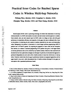
I. I NTRODUCTION Control theory deals with stabilizing and regulating the behavior of a dynamical system (“plant”) via real-time causal feedback. Traditional control theory was mainly concerned and used in well-crafted closed engineering systems, which are characterized by the measurement and control modules being co-located. The theory and practice for this setup are now well established; see, e.g., [1]. Nevertheless, in the current technological era of ubiquitous wireless connectivity, the demand for control over wireless media is ever growing. This networked control setup presents more challenges due to its distributed nature: The plant output and the controller are no longer co-located and are separated by an unreliable link (see Fig. 1). To stabilize an unstable plant using the unreliable feedback link, an error-correcting code needs to be employed over the latter. In one-way communications — the cornerstone of information theory — all the source data are assumed to be known in advance (non-causally) and are recovered only when the reception ends. In contrast, in coding for control, the source data are known only causally, as the new data at each time instant are dependent upon the dynamical random process. Moreover, the controller cannot wait until a large This work was supported in part by the National Science Foundation under grants CNS-0932428, CCF-1018927, CCF-1423663 and CCF-1409204, by a grant from Qualcomm Inc., by NASA’s Jet Propulsion Laboratory through the President and Directors Fund, and by King Abdullah University of Science and Technology.

block is received; it needs to constantly produce estimates of the system’s state, such that the fidelity of earlier data improves as time advances. Both of these goals are achieved via causal coding, which receives the data sequentially in a causal fashion and encodes it in a way such that the error probability of recovering the source data at a fixed time instant improves constantly with the reception of more code symbols. Sahai and Mitter [2] provided necessary and sufficient conditions on the required communication reliability over the unreliable feedback link to the controller. To that end, they defined the notion of anytime capacity as the appropriate figure of merit for this setting, which is essentially the maximal possible rate of a causal code that at any time t recovers a source bit at time (t − d) with error probability that decays exponentially with d, for all d. They further recognized that such codes have a natural tree code structure, which is similar to the codes developed by Schulman for the related problem of interactive computation [3]. Unfortunately, the result by Schulman (and consequently also the ones by Sahai and Mitter) only proves the existence of a tree code with the desired properties and does not guarantee that a random tree code would be good with high probability. The main difficulty comes from the fact that proving that the random ensemble achieves the desired exponential decay does not guarantee that the same code achieves this for every time instant and every delay. Sukhavasi and Hassibi [4] circumvented this problem by introducing linear time-invariant (LTI) tree codes. The timeinvariance property means that the behavior of the code at every time instant is the same, which suggests, in turn, that the performance guarantees for a random (time-invariant) ensemble are easily translated to similar guarantees for a specific code chosen at random, with high probability. However, this result assumes maximum likelihood (ML) decoding, which is impractical except for binary erasure channels (in which case it amounts to solving linear equations which has polynomial computational complexity). Sequential decoding was proposed by Wozencraft [5] and subsequently improved by others as a means to recover random tree codes with reduced complexity with some compromise in performance; specifically, for the expected complexity to be finite, the maximal communication rate should be lower than the cutoff rate. For a thorough account of sequential decoding, see [6, Ch. 10], [7, Sec. 6.9], [8, Ch. 6], [9, Ch. 6]. This technique was subsequently adopted by Sahai and Palaiyanur [10] for the purpose of decoding (time-varying) tree codes for networked control. Unfortunately, this result relies

wt

Plant

xt

vt

of matrices {Gt,i | i = 1, . . . , t ; t = 1, . . . , ∞} that provides anytime reliability. We recall this definition as stated in [4].

Sensor yt

Definition 1. Define the probability of the first error event as   ˆt−d|t , ∀δ > d, bt−δ = b ˆt−δ|t , Pe (t, d) , P bt−d 6= b

ct

ut Controller ˆ t|t x Fig. 1.

zt

Channel

Basic networked control system.

on an exponential bound on the error probability by Jelinek [11, Th. 2] that is valid for the binary symmetric channel (BSC) (and other cases of interest) only when the expected complexity of the sequential decoder goes to infinity [12]. In this work we propose the usage of sequential decoding for the recovery of LTI tree codes. To that end, similarly to Sahai and Palaiyanur [10], we extend a (different) result developed by Jelinek [6, Th. 10.2] for general (non-linear and time-variant) random codes to LTI tree codes. II. P ROBLEM S ETUP AND M OTIVATION We are interested in stabilizing an unstable plant driven by bounded noise over a noisy communication link. In particular, an observer of the plant measures at every time instant t a noisy version yt ∈ R (with bounded noise) of the state of the plant xt ∈ Rm . The observer then quantizes yt to bt ∈ Zk2 , and encodes — using a causal code — all quantized measurements {bi }ti=1 to produce ct ∈ Zn2 . This packet ct is transmitted over a noisy communication link to the controller, which receives z t ∈ Z n , where Z is the channel output alphabet. The controller then decodes {z i }ti=1 to produce the estimates ˆi|t }t , where b ˆi|t denotes the estimate of bi when decoded {b i=1 at time t. These estimates are mapped back to measurement estimates {ˆ yi|t }ti=1 which, in turn, are used to give an estimate ˆ t|t of the current state of the plant. Finally, the controller x ˆ t|t and applies it to computes a control signal ut based on x the plant. The need for causally sending measurements of the state in real time motivates the use of causal codes in this problem. Generally speaking, a causal code maps, at each time instant t, the current and all previous quantized measurements to a packet of n bitsct ,   t ct = ft {bi }i=1 . When restricted to linear codes, each function ft can be characterized by a set of matrices {Gt,1 , . . . , Gt,t }, where Gt,i ∈ Zn×k . The sequence of quantized measurements at 2 time t, {bi }ti=1 , is encoded as, ct = Gt,1 b1 + Gt,2 b2 + · · · + Gt,t bt . The decoder computes a function gt ({z i }ti=1 ) to produce {bi|t }ti=1 . One is then assigned the task of choosing a sequence

where the probability is over the randomness of the plant and the channel noise. Suppose we are assigned a budget of n channel uses per time step of the evolution of the plant. Then, an encoder–decoder pair is called (R, β) anytime reliable if there exists d0 ∈ N, such that Pe (t, d) ≤ 2−βnd ,

∀t, d ≥ d0 ,

(1)

where β is called the anytime exponent. According to the definition, anytime reliability has to hold for every decoding instant t and every delay d. Sukhavasi and Hassibi proposed in [4] a code construction based on Toeplitz block-lower triangular parity-check matrices, that provides an error exponent for all t and d. The Toeplitz property, in turn, avoids the need to compute a double union bound. We shall explicitly show this later in Section IV, where we introduce the LTI ensemble. In this work, the communication link between the observer and the controller is assumed to be a memoryless binaryinput output-symmetric (MBIOS) channel: w(zi |ci = 0) = w(−zi |ci = 1), where w is the channel transition distribution, zi ∈ Z and ci ∈ Z2 . III. P RELIMINARIES : C ONVOLUTIONAL C ODES In this section we review known result for several random ensembles of convolutional codes, in Section III-A. The codes within each ensemble can be either linear or not; linear ensembles can be further either time variant or time invariant. We further discuss sequential decoding algorithms and their performance in Section III-B which will be applied in the sequel for tree codes. A. Bounds on the Error Probability under ML Decoding We now recall exponential bounds for convolutional codes under certain decoding regimes. A compact representation (and implementation) of a convolutional code is via a shift register: The delay-line (shift register) length is denoted by d, whereas its width k is the number of information bits entering the shift register at each stage. Thus, the total memory size is equal to dk bits. At each stage, n code bits are generated by evaluating n functionals over the dk memory bits and the new k information bits. We refer to these n bits as a single branch. Therefore, the rate of the code is equal to R = k/n bits per channel use. In general, these functionals may be either linear or not, resulting in linear or non-linear convolutional codes, respectively, and stay fixed or vary across time, resulting in time-invariant or time-variant convolutional codes. We further denote the total length of the convolutional code frame upon truncation by N . Typically, the total length of the convolutional code frame is chosen to be much larger than d, i.e., N  d. We shall see

in Section IV, that in the context of tree codes, a decoding delay of d time steps of the evolution of the plant into the past corresponds to a convolutional code with delay-length d. Since each time step corresponds to n uses of the communication link, the relevant regime for the current work is N = nd. Theorem 1 ( [8, Sec. 5.6], [9, Sec. 4.8]). The probability of the first error event of random time-variant and LTI convolutional codes, under optimal (maximum likelihood) decoding, is bounded from the above by P¯e (d) ≤ 2−EG (R)nd

(2)

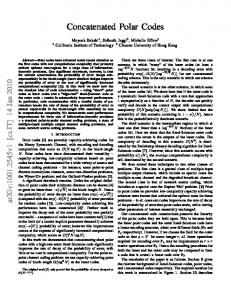
where EG (R) is Gallager’s error exponent function [7, Sec. 5.6], defined as (see also Fig. 2): EG (R) , max [E0 (ρ) − ρR] , (3a) 0≤ρ≤1 ( ) i1+ρ Xh 1 1 1+ρ 1+ρ (z|0) + w (z|1) E0 (ρ) , 1 + ρ − log w . z∈Z

(3b) We note that in the common work regime of N  d, the optimal achievable error exponent was proved by Yudkin and by Viterbi to be much better than EG (R) [8, Ch. 5]. Unfortunately, this result does not hold for the case of N = nd which is the relevant regime for this work. Interestingly, whereas time-variant codes are known to achieve better error exponents than linear time-invariant (LTI) ones when N  d, this gain vanishes when N = nd, as is suggested by the following theorem. Theorem 2 ( [13, Eq. (14)]). The probability of the first error event of LTI random convolutional codes, under optimal (maximum likelihood) decoding, is bounded from the above by (1). Thus, (1) remains valid for LTI codes. Unfortunately, the computational complexity of maximumlikelihood decoding grows exponentially with the delay-line length d, prohibiting its use in practice for large values of d. We therefore review next a suboptimal decoding procedure, the complexity of which does not grow rapidly with d but still achieves exponential decay in d of the BER. B. Sequential Decoding The Viterbi algorithm [8, Sec. 4.2] offers an efficient implementation of (frame-wise) ML1 decoding for fixed d and growing N . Unfortunately, the complexity of this algorithm grows exponentially with N when the two are coupled, i.e., N = nd.2 Prior to the adaptation of the Viterbi algorithm as the preferred decoding algorithm of convolutional codes, sequential decoding was served as the de facto standard. A wide class of algorithms fall under the umbrella of “sequential decoding”. Common to all is the fact that they explore 1 For

bitwise ML decoding, the BCJR algorithm [14] needs to be used. 2 This is true with the exception of the binary erasure channel, for which ML decoding amounts to solving a system of equations, the complexity of which is polynomial.

only a subset of the (likely) codeword paths, such that their complexity does not grow (much) with d, and are therefore applicable for the decoding of tree codes.3 In this work we shall concentrate on the two popular variants of this algorithm — the Stack and the Fano (which is characterized by a quantization parameter ∆) algorithms. We next summarize the relevant properties of these decoding algorithms when using the generalized Fano metric (see, e.g., [6, Ch. 10]) to compare possible codeword paths: M (c1 , . . . , cN ) =

N X

M (ct ),

(4a)

w(zt |ct ) − B, p(zt )

(4b)

t=1

M (ct ) , log

where B is referred to as the metric bias and penalizes longer paths when the metrics of different-length paths are compared. In contrast to ML decoding, where all possible paths (of length N ) are explored to determine the path with the total maximal metric,4 using the stack sequential decoding algorithm, a list of partially explored paths is stored, where at each step the path with the highest metric is further explored and replaced with its immediate descendants and their metrics. The Fano algorithm achieves the same without storing all these potential paths, at the price of a constant increase in the error probability and computational complexity; for a detailed descriptions of both algorithms see [6, Ch. 10], [7, Sec. 6.9], [8, Ch. 6], [9, Ch. 6]. The choice B = R is known to minimize the expected computational complexity, and is therefore the most popular choice in practice. Moreover, for rates below the cutoff rate R < R0 , E0 (ρ = 1), the expected number of metric evaluations (2) is finite and does not depend on d, for any B ≤ R0 [7, Sec. 6.9], [6, Ch. 10]. Thus, the only increase in expected complexity of this algorithm with d comes from an increase in the complexity of evaluating the metric of a single symbol (2). Since the latter increases (at most) linearly with d, the total complexity of the algorithm grows polynomially in d. Furthermore, for rates above the cutoff rate, R > R0 , the expected complexity is known to grow rapidly with N for any metric [12], implying that the algorithm is applicable only for rates below the cutoff rate. Most results concerning the error probability under sequential decoding consider an infinite code stream (over a trellis graph) and evaluate the probability of an erroneous path to diverge from the correct path and re-merge with the correct path, which can only happen for N > nd. Such analyses are not adequate for our case of interest, in which N = nd. The following theorem provides a bound for our case. Theorem 3 ([6, Ch. 10]). The probability of the first error event of general random convolutional codes, using the Fano 3 Interestingly, the idea of tree codes was conceived and used already in the early works on sequential decoding [5]. These codes were used primarily for the classical communication problem, and not for interactive communication or control. 4 Note that optimizing (2) in this case is equivalent to ML decoding.

Exponent

0.3

Sec. 6.9] for LTI convolutional codes; for both, delay-line length d is assumed to be infinite.7

EG (R) EJ (B = R0, R) EJ (B = R, R) EG (R)/2 Capacity R0

0.2

0.1

0 0

0.1

0.2

0.3

0.4

Theorem 4. The probability that Wt of a general random convolutional code or an LTI convolutional code with infinite delay-length is larger than m ∈ N is upper bounded by 0.5

R [bits]

Pr (Wt ≥ m) ≤ Am−ρ , where A is finite for B, R < R0 , R
0. 6 For finite values of d a lower choice of B might be better, since the constant A might be smaller in this case.

Pr (Wt ≥ m) ≥ (1 − o(m))m−ρ , where o(m) → 0 for m → ∞, and R =

E0 (ρ) ρ

and any ρ > 0.8

This result was proved to be tight by Savage [15] for general random convolutional code, and is widely believed to be true for random LTI convolutional codes, although no formal proof exists for the latter. IV. L INEAR T IME I NVARIANT A NYTIME R ELIABLE C ODES In this section, we recall the construction of LTI anytime reliable codes as presented in [4]. A causal linear timeinvariant code has a parity-check matrix with the following lower triangular Toeplitz structure. The generator matrix of an (n, R) LTI code of rate R and blocklength n per time step is given by c = Gn,R b, where       b1 G1 0 ··· ··· ··· c1  b2  G2 c2  G 0 · · · · · · 1         ..   ..  ..  .. .. ..      . . · · ·, b =  . , c =  . Gn,R =  . .  bt   Gt Gt−1 · · · G1 0   ct        .. .. .. .. .. .. .. . . . . . . . (7) and Gt ∈ Zn×k . The following definition, given in [4], 2 dictates the way to choose the Gi ’s. Definition 3 (LTI Ensemble). Fix G1 to be a full rank matrix, and generate the entries of Gt independently and uniformly at random, for t ≥ 2. For the purpose of this paper, we shall view an (n, R) LTI code as a convolutional code with infinite delay-line length, k information bits and n code bits. As a result of this 7 For finite delay-length convolutional codes, the computational complexity can only be smaller than that of infinite delay-length codes. 8 Recall that E (ρ)/ρ is a decreasing function of ρ and therefore ρ > 1 0 implies that R < R0 .

interpretation, the results of Section III apply directly to this Toeplitz ensemble. We shall now show why such a construction does indeed guarantee anytime reliability as defined in (1). By using the Markov inequality along with the result of Theorem 1, the probability that a particular code from this ensemble has an exponent that is strictly smaller than (EG (R) − ) is bounded from the above by   P Pe (d) > 2−(EG (R)−)nd ≤ 2−nd . (8) Thus, for any  > 0, this probability can be made arbitrarily small by taking d to be large enough. However, for a code to be anytime reliable it needs to satisfy (1) for every t and d0 ≤ d ≤ t. Unfortunately, applying the union bound and (IV) to ! ∞ [ t n o [ −(EG (R)−)nd P Pe (t, d) > 2 t=1 d=d0

gives a trivial upper bound. The advantage of using an LTI code  is that for a fixed d, the event Pe (t, d) > 2−(EG (R)−)nd is identical for all t. Therefore, for LTI codes, we have ! t n ∞ [ o [ −(EG (R)−)nd Pe (t, d) > 2 (9a) P t=1 d=d0 ∞ n [

=P

−(EG (R)−)nd

Pe (t, d) > 2

! o

(9b)

d=d0

≤ =

∞ X

2−nd

d=d0 −nd0

2 . 1 − 2−n

(9c) (9d)

As a result, a large enough d0 guarantees that a specific code selected at random for the LTI ensemble achieves (1) with exponent β = (EG (R) − ), for all t and d0 ≤ d ≤ t, with high probability. V. S EQUENTIAL D ECODING OF L INEAR T IME -I NVARIANT A NYTIME R ELIABLE C ODES In this section we show that the upper bound on the probability of the first error event under sequential decoding for convolutional codes (3), holds true also for LTI convolutional codes, which for N = nd, identifies with the LTI tree codes of (IV). To prove this, we adopt the proof technique of [7, Sec. 6.2], where the exponential bounds on the error probability of random block codes are shown to hold also for linear random blocks codes. Theorem 6. The probability of the first error event of the LTI random tree ensemble of Definition 3, using the Fano or stack sequential decoders and the Fano metric with bias B, is bounded from the above by (3).

Proof sketch: A thorough inspection of the proof of Theorem 3, as it appears in [6, Ch. 10], reveals that the following two requirements for this bound to be valid are needed: 1) Pairwise independence. Every two paths are independent starting from the first branch that corresponds to source branches that disagree. 2) Individual codeword distribution. The entries of each codeword are i.i.d. and uniform. We next show how these two requirements are met for the affine linear ensemble. The codes in this ensemble are as in (IV) up to an additive translation v =  T v 1 v 2 · · · v t · · · , where v t ∈ Zn2 , with c = Gb + v. The entries of G and v are sampled independently and uniformly at random. ˜ are identical Now, assume that two source words b and b ˜i for i < t and differ in at least one bit in branch t, i.e., bi = b ˜ for i < t and bt 6= bt . Then, the causal structure of G ˜t ˜i for i < t. Moreover, bt 6= b guarantees that also ci = c along with the random construction of  G suggest that T the two code paths starting from branch t, cTt cTt+1 · · · and  T T ˜t c ˜Tt+1 · · · are independent. This establishes the first c requirement. To establish the second requirement we note that the addition of a random uniform translation vector v guarantees that the entries of each codeword are i.i.d. and uniform. This establishes the second requirement and hence also the validity of the proof of [6, Ch. 10]. Finally, note that since the channel is MBIOS, the same error probability is achieved for any translation vector v. Since Theorem 6 holds for LTI codes, a specific code chosen from the LTI ensemble is anytime reliable with (3), with high probability, following (4). VI. S IMULATION OF A C ONTROL S YSTEM To demonstrate the effectiveness of the sequential decoder in stabilizing an unstable plant driven by bounded noise, we simulate a cart–stick balancer controlled by an actuator that obtains noisy measurements of the state of the cart through a BSC. The example is the same one from [4] which is originally from [16]. The plant dynamics evolve as, xt+1 = Axt + But + wt yt = Cxt + vt , where ut is the control input signal that depends only on the estimate of the current state, i.e. ut = Kˆ xt|t . The system noise wt is a vector of i.i.d. Gaussian random variables with mean µ = 0 and variance σ 2 = 0.01, truncated to [−0.025, 0.025]. The measurement noise vt is also a truncated Gaussian random variable of the same parameters. We assume that the system is in observer canonical form:     3.3010 1 0 −0.0300   A = −3.2750 0 1 , B = −0.0072 , C = 1 0 0 , 0.9801 0 0 0.0376

TABLE I AVERAGE LQR C OST OVER 100 CODES WITH 40 EXPERIMENTS PER CODE

Cart Stick Balancer - Angle n = 20 LTI Code over BSC(0.01)

15

R= R=

1 2 1 5

k 4 5 10

Angle θ (degrees)

10

LQR Cost 206.0 86.4 873.0

5

0

−5

−10

0

50

100

150

200 Time t

250

300

350

400

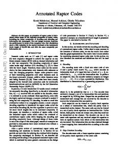
Fig. 3. Stability of the Cart–Stick Balancer is demonstrated using a sequentially decoded LTI code.

 K = −55.6920

−32.3333

 −19.0476 .

The state xt , before the transformation to observer canonical form, is composed of the stick’s angle, the stick’s angular velocity and the cart’s velocity. The system is unstable with the largest eigenvalue of A being 1.75. The channel between the observer and the controller is a BSC with bit-flip probability p = 0.01, which has a cutoff rate R0 = 0.7382. We fix a budget of n = 20 channel uses. Using Theorem 8.1 in [4], the minimum required number of quantization bits is kmin = 3 and the minimum required exponent is βmin = 0.2052. For the first experiment, we use a code of rate R = 1/2, with k = 10 bits for a lattice quantizer with bin width δ = 0.1. From (3), a sequential decoder with bias R0 will guarantee an error exponent of β = 0.2382. As is evident from the dark curve in Fig. 3, the stick on the cart does not deviate by more than 12 degrees. For the second experiment, we use a lower code rate R = 1/5, which provides β = 0.5382. The light curve in Fig. 3 shows that the deviation is reduced to 4 degrees. Although these simulations might suggest that a lower rate code always results in better stability of the dynamical system, it is not a-priori clear that this is truly the case. A lower code rate uses a coarser quantizer than a higher rate code. As a result, there could be some loss due to this coarseness. A common metric used to quantify the performance of the closed-loop stability of a dynamical system is the linear quadratic regulator (LQR) cost for a finite time horizon T given by " # T  1 X 2 2 J =E kxt k + kut k , 2T t=1 where the expectation is w.r.t. the randomness of the plant and the channel. For our example, we simulated the system using three different quantization levels, with 100 codes per quantization level and 40 experiments per code. The data is tabulated in Table I.

In principle, one would randomly sample an LTI generator matrix where each subblock Gi ∈ Zn×k . Nonetheless, from 2 an implementation efficiency point of view, there0 is0 no loss in the anytime exponent if we pick Gi ∈ Zn2 ×k , where n = n0 gcd(n, k) and k = k 0 gcd(n, k), and then using the first tgcd(n, k) blocks to encode {bi }ti=1 . VII. D ISCUSSION We showed that sequential decoding algorithms have several desired features: Error exponential decay, memory that grows linearly (in contrast to the exponential growth under ML decoding) and expected complexity per branch that grows linearly (similarly to the encoding process of LTI tree codes). However, the complexity distribution is heavy tailed (recall Theorems 4 and 5). This means that there is a substantial probability that the computational complexity is going to be very large, which will cause, in turn, a failure in stabilizing the system. Specifically, by allowing only a finite backtracking length to the past, the computational complexity can be bounded at the expense of introducing an error due to failure. From a practical point of view, the control specifications of the problem determine a probability of error threshold under which a branch ct is considered to be reliable. This can be used to set a limit on the delay-line length of the tree code, which in turn converts it to a convolutional code with a finite delay-line length. Finally, note that tighter bounds can be derived below the cutoff rate via expurgation. Moreover, random linear block codes are known to achieve the expurgated bound for block codes (with no need in expurgation) [17]. Indeed, using this technique better bounds under ML decoding were derived in [4] and a similar improvement seems plausible for sequential decoding. VIII. ACKNOWLEDGMENTS We thank R. T. Sukhavasi for many helpful discussions and the anonymous reviewers — for valuable comments. R EFERENCES [1] B. Hassibi, A. H. Sayed, and T. Kailath, Indefinite-Quadraric Estimation and Control: A Unified Approach to H2 and H-infinity Theories. New York: SIAM Studies in Applied Mathematics, 1998. [2] A. Sahai and S. K. Mitter, “The necessity and sufficiency of anytime capacity for stabilization of a linear system over a noisy communication link—part I: Scalar systems,” IEEE Trans. Inf. Theory, vol. 52, no. 8, pp. 3369–3395, Aug. 2006. [3] L. J. Schulman, “Coding for interactive communication,” IEEE Trans. Inf. Theory, vol. 42, pp. 1745–1756, 1996. [4] R. T. Sukhavasi and B. Hassibi, “Error correcting codes for distributed control,” IEEE Trans. Auto. Control, accepted, Jan. 2016. [5] J. M. Wozencraft, “Sequential decoding for reliable communications,” Res. Lab. of Electron., Massachusetts Institute of Technology, Cambridge, MA, USA, Tech. Rep., 1957.

[6] F. Jelinek, Probabilistic Information Theory: Discrete and Memoryless Models. New York: McGraw-Hill, 1968. [7] R. G. Gallager, Information Theory and Reliable Communication. New York: John Wiley & Sons, 1968. [8] A. J. Viterbi and J. K. Omura, Principles of Digital Communication and Coding. New York: McGraw-Hill, 1979. [9] R. Johannesson and K. S. Zigangirov, Fundamentals of Convolutional Coding. New York: Wiley-IEEE Press, 1999. [10] A. Sahai and H. Palaiyanur, “A simple encoding and decoding strategy for stabilization discrete memoryless channels,” in Proc. Annual Allerton Conf. on Comm., Control, and Comput., Monticello, IL, USA, Sep. 2005. [11] F. Jelinek, “Upper bounds on sequential decoding performance parameters,” IEEE Trans. Inf. Theory, vol. 20, no. 2, pp. 227–239, Mar. 1974. [12] E. Arıkan, “An upper bound on the cutoff rate of sequential decoding,” IEEE Trans. Inf. Theory, vol. 34, no. 1, pp. 55–63, Jan. 1988. [13] N. Shulman and M. Feder, “Improved error exponent for time-invariant and periodically time-variant convolutional codes,” IEEE Trans. Inf. Theory, vol. 46, pp. 97–103, 2000. [14] L. Bahl, J. Cocke, F. Jelinek, and J. Raviv, “Optimal decoding of linear codes for minimizing symbol error rate,” IEEE Trans. Inf. Theory, vol. IT-20, pp. 284–287, Mar. 1974. [15] J. E. Savage, “Sequential decoding — the computation problem,” Bell Sys. Tech. Jour., vol. 45, no. 1, pp. 149–175, Jan. 1966. [16] G. Franklin, J. D. Powell, and A. Emami-Naeini. New Jersey: Pearson Prentich Hall, 2006. [17] A. Barg and G. D. Forney Jr., “Random codes: Minimum distances and error exponents,” IEEE Trans. Inf. Theory, vol. 48, no. 9, pp. 2568–2573, Sep., 2002.