namely: water body covered by a layer of ice--winter period, completely mixed water body--spring and autumn periods, stable thermic stratification of the water ...
Ecological Modelling, 26 (1984) 77-96
77
Elsevier Science Publishers B.V., Amsterdam - Printed in The Netherlands
A COMPREHENSIVE SENSITIVITY ANALYSIS FOR AN ECOLOGICAL SIMULATION MODEL
FRIEDER RECKNAGEL
University of Technology, Water Resources Department, Laboratory of Hydrobiology, Dresden (German Democratic Republic)
ABSTRACT Recknagel, F., 1984. A comprehensive sensitivity analysis for an ecological simulation model. Ecol. Modelling, 26: 77-96. A comprehensive sensitivity analysis was carried out for the ecological simulation model SALMO. By means of an analytical approach the relative model sensitivity is investigated and evaluated against changing parameters, changing the input discretization interval, changing initial conditions of the state variables, randomly perturbed rate variables and various numerical integration methods to solve the differential equations. Because of the large number of parameters in ecological models a strategy which seeks the shortest way for the highest parameter sensitivity is introduced by hierarchical decomposition of the parameter file into macroparameters according to state, rate and auxiliary variables. The parameter sensitivity determined in this way is compared with the relative variance of parameter estimates to indicate directions for future research. The relative sensitivity is presented by the polar coordinate method.
INTRODUCTION
Along with simulation modelling the importance of methodology for model validation and evaluation increases. Within such a methodology, sensitivity analysis appears as a powerful tool (Ford and Gardiner, 1979; Sargent, 1979; Swartzman, 1980; Majkowski et al., 1981; Recknagel and Benndorf, 1982). Sensitivity analysis is generally divided in two different approaches: analytical and numerical. The numerical approach was founded by Tomoviz and Vukobratovic in 1972 and their work initiated many papers. The analytical approach has been executed by numerous techniques. This author agrees with Halfon (1977) and Swartzman (1980) that the numerical approach is inducing numerical errors of approximation and is too complicated 0304-3800/84/$03.00
© 1984 Elsevier Science Publishers B.V.
78 to make a comprehensive analysis of the complex simulations required of ecological models. Sensitivity analysis for the ecological simulation model SALMO is carried out in an analytical approach using the polar coordinate technique (Thornton et al., 1979; Recknagel, 1980). It considers: parameter sensitivity, sensitivity against the input discretization interval, initial condition sensitivity, sensitivity against randomly perturbed rate variables and numerical integration method sensitivity. Analysis of parameter sensitivity of SALMO includes a strategy which seeks the shortest way for the highest sensitivity within the 83 parameters. The strategy is based on a hierarchical decomposition of the macroparameters which are assigned endogenous system quantities: state variables, rate variables (absolute rates) and auxiliary variables (including relative rates). The parameter sensitivity determined in this manner is compared with the relative variance of parameter estimates to identify directions for future research. SENSITIVITY ANALYSIS In the context of this paper sensitivity analysis is used in the ecological simulation model SALMO for the management of lakes and reservoirs (Benndorf, 1979; Recknagel, 1980, 1984). It involves the following state variables: phytoplankton X1 (microplankton diatoms), phytoplankton X2 (green algae and nanoplankton diatoms), herbivorous zooplankton Z, dissolved orthophosphate P, dissolved inorganic nitrogen N and dissolved oxygen O. The influence of fishes upon zooplankton mortality at present is taken into account implicitly by constant parameters. The input file of SALMO contains the decade means of 19 hydrological, meteorological and physical driving variables which are interpolated linearly or stochastically, depending on their nature. By reason of SALMO's primary application in decision making for eutrophication control (Benndorf and Recknagel, 1982; Recknagel, 1984). its sensitivity under conditions of a very high nutrient load is worth knowing. Therefore the annual cycle of the state variables mentioned above is investigated for the multi-purpose hypereutrophic Bautzen reservoir on the basis of the input file for the year 1978. Method
The polar coordinate technique enables the investigator to yield compact plots of the relative model sensitivity where the day-by-day comparison of a reference standard simulation run and a perturbed simulation run for any
79 endogenous system quantity is made (Figs. 1 13). The reference simulation run is represented as a dotted unit circle. Using the 360 ° of the unit circle the daily model sensitivity of one simulated year can be considered where the maximal sensitivity displayed by the plots amounts to 100%. In addition to the daily sensitivity the seasonal sensitivity is also represented in the plots. However, the seasonal periods of a year simulated by SALMO are individually defined for each year and are time specific for the ecosystem under consideration depending on hydrophysicai conditions, namely: water body covered by a layer of ice--winter period, completely mixed water body--spring and autumn periods, stable thermic stratification of the water b o d y - - s u m m e r period. To each sensitivity plot, which refers to a specified state variable, is added a tabled, precise numerical sensitivity crest factor for each season.
Parameter sensitiuity The highly complex behaviour of aquatic ecosystems requires an extensive endogenization of causal relationships of the system behaviour into ecosystem models. Such an endogenization, however, causes a disadvantageous increase of the model structure and especially of the number of parameters. SALMO seems to be a reasonable compromise between the necessary minimum of state variables and the maximal endogenization of ecosystem behaviour (Benndorf and Recknagel, 1982). Nevertheless SALMO involves 83 constant parameters which are estimated on the basis of field and laboratory experiments (Benndorf, 1979). Because it would be too expensive to check the model sensitivity for each of the 83 parameters the researchers have followed a seeking strategy for the highest parameter sensitivity using hierarchically decomposed macroparameters. Figures 1 and 2 show the state variable sensitivity with respect to a change by _+5% of the macroparameters which are assigned to the state variables. The sensitivity attained a magnitude of up to 454% of phytoplankton X1 against changing its macroparameter X1 by - 5 % (Fig. 1, left); hence, in the next step sensitivity of phytoplankton X1 against the macroparameters which are assigned the rate variables (growth, grazing by zooplankton and sedimentation of X1) was considered with the same change of - 5 % (Fig. 3). By reason of the dominance of the sensitivity of X1 against the macroparameter referred to as the growth rate (181%; Fig. 3, left) it was split into the macroparameters of the auxiliary variables (gross-photosynthesis and respiration). As a result of checking the sensitivity of X1 against a change by 5% of the macroparameters (Fig. 4) it can be seen that the influence of the respiration macroparameter clearly dominates (139%; Fig. 4, right). Among the four single constant parameters of the respiration macroparameter, the -
".
•
[1(1)3~1] PRY = EH DRY = [] DRY= 13E PRY= IZ3 DRY:ZZ'7
.°
5.i.: g.gl, 5~ix=Z~'l.Si,
DRY= I PRY=ZSB
5.nx = ~"tl.3 i t PRY : ~
5.1N= 9 , 9 Z / 5~x= 3Z.31/ S.l.= H.4•, S~mx= 11(3.71, Sam= L 3 1 , "
Xl
PHYTOPLANKTOH X1
.
•
t
i
.j. ~, " °,
,
..l,.
5.*.= g . g i , PRY: I 5rex= na.4S t PRY=252
5.ax = 411.3 i , PRY = ZH[
5.1a= ZZ.I I / DRY = 531 5m~x= H"I.S t , PRY= [] S.l.: 3 . 2 1 , PRY= IgB 5 ~ x = 5 9 . 3 I , PRY= IZ5 5.in= g . Z l , PRY= 153
XZ [1(1)~]
PHYTDPLBNKTONX2
.
%. ~ .
.~.:
%
I
• "H3lnam
;
, "~
33.2 S , DRY = 225
DRY = [] DRY= 5:1 PRY= 133 DAY= trio DRY= 197
.
1 H)I
m
356 [01
S.l.= g . g i , PRY= I Smoc= 53.S• , PRY =ZgB
S.nx =
Saza= Ig.GZ / S . ~ = IH.I I , 5.i.= g.gi, Sm~x= ~ . 9 I ; 5aiN= 9 . 3 I ,
7, [1{1)Z]]
Z00PLHNKTDNZ
L..." ,>..,.j
• .jll3mlns ,
""'''"'°)'"
Fig. 1. Parameter sensitivity ( S ) of the ecological model SALMO related to: phytoplankton biomass X1 against the macroparameter X1 of X1 (left); phytoplankton biomass X2 against the macroparameter X~ of X2 (middle); zooplankton biomass Z against the macroparameter Z of Z (right).
-BUTI]HH-
-5UHHER-
-SPRING-
-HINTER-
HHCHI]PitHItflETER
:l: [ % OF THE
FiT H CHI~IGE iSY
SENSITIVITY S DF :
.'
,.~.
." ' ¢. * . • , t ." ° '.
t•.
g.H ~ ~ B.B ~ ~ B.B~I ~ tl.G 3 ~ I;.2 ~I ~ lK.4~I ~ a.li%~ Iq.I II~
l)lqY = SB DRY = KB DflY = 7g DRY = 123 DRY = lql; DRY =216 DRY = I DflY=2Kit
I[P] 366 tD]
StuN= B.1% ~ DRY = SB c;.Rx = B.2 ~ , DRY = E;~] c;m. = H.2 % ~ DflY = 7B C;.RX = 2.H % t DRY = 121 c;m,= I.q ~I t DFIY = IHB 5HRX= 12.1% t DRY =212 5.1,= B . B ~ t DHY= I 5~RX= IB.2:I~ DRY=2KI
N [I(I)B]
P [I(I)~]
SHIN= S~x= ShiN= SHRX = 5raN= Snsx= 5,1N= S.nx=
NITRDSENN
PHfl.SPHBTEP
~
"
StuN= C;.RX= 5ran= 5.RX = 5,IN= 5~x= S,l.= S~mx=
D [I(I)31
DXYfEN
B.B' I , DRY = B.I ~1 ~ DRY = B.It ~1 ~ DRY = B.B % , DAY = B.H I / DflY = B.B ~ ~ DflY = B.B~ t DBY= B.B % ~ DRY=
I tD]
~B I;B 7H 7B IHB IqB I I
3GH t~]
Fig. 2. Parameter sensitivity (S) related to: dissolved orthophosphate P against the macroparameter P of P (left); dissolved inorganic nitrogen N against the macroparameter N of N (middle); dissolved oxygen O against the macroparameter O of O (right).
-BtlTLIHN-
-SLIltMER-
-~;PRINI:;-
-HINTER-
SENSITIVITY S DF : BT B CHBNBEBY ~ ~ UF THE MBCRUPBRBMETER =
36B CD]
¶ [D]
0,0
SMiN=
5NRX= fiH=,= 5,nx: S,l,= finnx= SMIN= 5,Frx=
~il
DRY = 69 DRY = 139 DRY = 115 DFIY=2~lfi DRY =219 DRY =23B DRY =322
9.E %,' DFIY:
13.2 % ~ 4.E % t 22,Bit B.7 %~ E.EII 1.7%~ 11.7 %,'
1 [DI 3611[DI
Fig. 3. Parameter sensitivity ( S ) related to: phytoplankton biomass X1 against the macroparameter GROWTH (growth rate of phytoplankton X1) (left): phytoplankton biomass X1 against the macroparameter G R A Z I N G (loss rate of phytoplankton X1 by zooplankton grazing) (middle): phytoplankton biomass X1 against the macroparameter SEDIMENTATION (sedimentation rate of phytoplankton X1 (right).
-RLITLIHN-
-5LJMHER-
-SPRINI;-
5~mx= 7.3%t 5aZN= 7,E% t 5~mx= 112.9~t tim,= B.HZt 5anx= IBl.3%t StuN= B.B%I ~ q x = 15:B.:3%/
5MIN: I.I ~,, DFJY: ~:B 5HRX= B.E ~ ~ DRY= fi9 fi,lN= B.B % t DRY = 7B 5 , , x = 37.7:~,. DRY= 12E 5,t,= B . B ~ t DRY= I ~ 5Max= I ~ . l ~ t DRY = lB7 StuN= B . B ~ t DRY= l SMax= i ~ . 4 ~ t DRY=2S7
5MIN:
-HINTER-
4.P1% t DRY :
fiEI)IMENTBTII]N [ I ( I ) I ]
fiRRZINB [1(1)13]
IP) 36JtLDI
fiRDWTH CI(I)20]
,,':
...~
PHYTDPLFINKTDNXl
.
PHYTDPLFINKT]]N11
5:R PRY = 1~9 ]}BY = 7B DRY = 131 DRY= 194 DRY =22B DRY= I DRY=2SB
e
°
PHYT[]PLRNETDI(11
o,
./
........
~
,.,'",*i,
5ENflTIYITY 5 DF BT B CHRNBEBY - K ~ OF THE HBCRDPBRBHETER
.
°.,
,.a.
OC I',J
I9.B ~ , DRY = 323
5~,x =
EB G~ IHI 123 Iq9 lEG I
3.G % , 4.SSt il.H % , G.BII, H.I ~ , IG.]~," g.B~[,
SHIN= 5.RX= SMz,= 5~x= 5.zN= SM~x= 5MZN=
DRY = DAY = DAY = DAY= DRY = DRY = DRY =
II.7 g , 22.3~, 2~].1 ~," IBG.21t, B.2 Z / IBS.~," B.B~,
DRY = DAY= DAY = PAY= DAY = DRY= DAY =
I
~R
1 [D]
7B 12] IRE IHB I SNex = 1395 % , DRY = 2SB
SNIN= SMnx= 5~ZN= 5~x= 5.zN= 5~x= 5MZN =
RESPIRATION [1(1)H]
PHDTOSYNTHESIS [ 1 (1117 ]
"" . . . . . . . . . . ""
$,
PHYTDPLRNk'TDN X1
~'t ;
',~'
e
PHYTOPLANKTDN Xl
("
.~
""'t ~, ~'•
" ""';....
."
Fig. 4. Parameter sensitivity (S) related to: phytoplankton biomass X1 against the macroparameter PHOTOSYNTHESIS (gross-photosynthesis rate of phytoplankton X1) (left); phytoplankton biomass X1 against the macroparameter RESPIRATION (respiration rate of phytoplankton X1) (right).
-RLITilMN-
-SIIHHER-
-SPRING-
-HINTER-
SENSITIVITY S DF : AT R CHANGE 6Y - E ~ OF THE NRCROPRRRMETER :
:t~ [D'J
1 (,P]
.
......._i ~
p,..J
S,RX= 21.q I i DRY=2~
I
[)BY=219
fl.B][,' DRY=
5,,x=
S,z.=
S,RX=
5Nex= 5,ZN=
5,1.=
S.RX:
5.1.=
RXTHINI
PRY= I ~
I q.7 Z i DRY = q9
B.i]!~ DRY=
i.91t
G.I Z , DRY= GEl 1 . 2 I , ' DFiY= 139 El.I | ~ DRY = 114 ll.~lZ, DRY= IFE
LI.F;I~ DFIY :
PHY'mPL~KTnN Xl
Fig. 5. Parameter sensitivity (S) related to: phytoplankton biomass X1 against the constant parameter I O P I X I (optimum water temperature for growth of phytoplankton X1) (left); phytoplankton biomass X1 against the constant parameter RXMF1 (proportion of the grossphotosynthesis rate of X1 lost by respiration) (middle); phytoplankton biomass XI against the constant parameter RXTM1N1 (minimal respiration rate of X1 at a temperature near 0 o C) (right).
] 9 . 7 1 i DRY = 2 ~
5.,x=
S,z.=
El,FIX= 1 7 . B I /
I
DRY= 199
il.BI," ])fly =
5,m=
5:.2~, [)FLY= 7B
Smlx= " i l . 9 I i
-RUTLINN-
S.t,=
-SilliER-
7B
[;mix= IE;,EII~ DRY = 121 S,z, '~ B . 6 : i l ])BY= IE9
"t.I I ~ DRY :
5,1.=
I)flY= [ ]
S~:lx= 23.41,' DRY: 121 5raN= i , i Z t DFIY= II;B
E,I I ,
-SPRING-
5.FIx:
3.1l~t, DHY= Kil
I.Klt
],t]~It DFIY: GEt
S.tN=
5~x:
-MINTER-
S.IN=
RXHF1
TllOTXI DFI¥ = KB
PHYT[]PLflNKTDNXI
PHYTI1~.RNKT['INXl
ENSITIVITY 5 OF " RT R CHRltE -E~ DFTHE (~lST. PRRRNETER :
1 [P]
oo
85 TABLE I Comparison of the relative variance of parameter estimates (Benndoff, pers. comm.) and the maximal parameter sensitivity of phytoplankton X1 related to the parameters TOPTX1, RXMF1 and RXTMIN1 (cf. Fig. 5) Constant parameter
Relative variance of parameter estimates (%)
Maximum parameter sensitivity of )(1 (%)
TOPTX1 RXMF1 RXTMIN1
25 80 70
39.7 41.4 9.1
parameter TOPTX1 (optimum water temperature for growth of phytoplankton X1) induces the highest sensitivity in X1 at a change of - 5 % (40%; Fig. 5, left). Table I contains the comparison between the relative variance of parameter estimates and the maximal parameter sensitivity related to the constant parameters TOPTX1, RXMF1 (proportion of the gross-photosynthesis rate of X1 lost by respiration) and RXTMIN1 (minimal respiration rate of X1 at a temperature near 0°C) for which the highest parameter sensitivity of phytoplankton X1 was determined (Fig. 5). TOPTX1 has a low relative variance but induces the highest parameter sensitivity of X1. The estimate of RXMF1 exhibits the highest relative variance and causes a high parameter sensitivity of X1. Finally the relative variance of the estimated magnitude of RXTMIN1 is high but the resulting parameter sensitivity in X1 is the lowest. Future experimental efforts should be concentrated on the minimization of the variance of parameter estimates of TOPTX1 and RXMF1 by investigating them particularly in seasons of their highest parameter sensitivity on X1 (summer and autumn). Within the reduced variances it is useful to determine the new parameter estimates for the model by using an appropriate parameter optimization procedure (Recknagel and Benndorf, 1982). In this manner the parameter sensitivity of each state variable of a model should be determined and interpreted to improve the parameter reliability and the model validity.
Sensitivity against input discretization interval There are two ways of considering the driving variables in ecological models. The first one is endogenization using of trigonometric, respectively polynominal, functions to generate smooth time series for a typical year and system. In the second way the discrete mean values of actual measurements are used to observe the model's response to actual crest factors in hydrologi-
" " .'"
:.
"t-.
":" .'.,~.. • •
5a~: 5.m : 5.t.= 5..x=
5.iw=
5.z.= DFIY=175
DFIY=t7E
....
.'
5.21, IB.B I 1.7 I 39.q I i i.t I 1t3.5 I II.iI, qT.~l,
\
|
DRY = 5G , DRY = "7B t DRY =t34 DflY =tEE ~ DRY :2~B , DRY : 1fll DflY = '1 DflY=29"7
% l.
- ,,, ~,.. .~,
ZDDPLBNKTDNZ
•:::
:
.... ~ - ~
DflY =IB6
....
S.t.= E;,~=
I[D]
64 ~
DRY= DRY=
Oo
DRY : t74 DRY= 'I S.m = BB.4 i , DRY = 2BK
SxtN= 4 2 . 2 I ~ Snnx= 7 B . f l ~ , 5NiW= B.E %, 5nmt=~.t 1," 5.i.: 4.1 l , 5.mr : 'I]7.B % , 5.IN= B.il,
PHYI'I]PL~KTDNX~
..
~ ,~-, ,,~
"1-.
-#. ~N.,,~-.
..'~'7,-- ....
-..~ ,.~
"
. . . , .::"
./.%
"".":"{ •,~i~
•.
•
'I [D]
Fig. 6. I n p u t discretization sensitivity ( S ) related to: p h y t o p l a n k t o n b i o m a s s XI (left): p h y t o p l a , ~ k t o n b i o m a s s X2 (middle): z o o p l a n k t o n b i o m a s s Z (right).
5 ~ x = 9tl.B % , DFIY = 31G
5 am( = 975.2 I / DflY = 177 5ran= B.! I i DRY = 1
DflY=2EB
-FIUI"].IHN-
B.2lt
DIqY = t~G DflY ='1]'7 DAY = ~]-~ DBY = 17_.5
5MiN=
5.IN= t;.fi %,' SH,X= 1 1 . ~ 3 I SHIN = B.~" ~ , 5 . . x = 21~.9 I t
-51.1HH~-
- 5Pl~lNfi -
-NIN]'~-
"..../"
..
.*'.
.
[D'I
:.
.,'
...-,, t.
.~ ":v-,,-'---:."
/
,,
,,,
SMR~X =
5.ex= 5m.=
5mN=
5,RX=
5raN= 5,.x= 5.m=
1 [D3 3611 [P]
2fi.fl % , PRY = ZS7
Sfl.q ¢ , DRY = 219 B.11 1," DRY =27B
11.11%, DRY = I %
23.1t %, PflY = 123
I.q ~ , DRY = El q.q Z , PRY = SI B.It I , PflY = 13:1
5EDIMENTBTIDN
PHYT1]PLRNKTflN Xl
.];t
Fig. 9. Sensitivity (S) against randomly perturbed rate variables related to: phytoplankton biomass XI against the rate variable GROWTH (growth rate of X1) (left); phytoplankton biomass X1 against the rate variable G R A Z I N G (loss rate of X1 by zooplankton grazing) (middle): phytoplankton biomass X1 against the rate variable SEDIMENTATION (sedimentation rate of X1) (right).
= 127.1 I , DRY = 311K
-RUTUHN-
5~x
73.11%, DRY = IF;il B.B I , " DRY = 33
5.~= 5.=.=
DFIY = lfi4
qZ.7 I t DFIY = 13fl
5.R'X= B.I 1 ,
Pl.1%, DRY = F;H K.I I , DRY = GB 01.3 %, DflY = 75
5.IN= 5NP.X= StuN=
GRDWTH
-
3GB [p]
5mN=
:
= PHYTDPLRNKTDNXl
,-"
,, ,"
~,
-5UHHER-
- SPRING-
-WINTER-
fiT R PSEUDD-RBNDDMLY PERTURBBTIDNBY ~ [@ I OF THE RBTEVBRIFIBLE
5EN51TIVITY S DF
:
°• " . ~ , • l • , o., • .°'o •
, .::..:'~
.,:,-" ~
,.:.,,,,,-rn
DRY = DRY = DRY = DRY= DRY =
B.7 X ~ DRY =
5r~Rx= 79.9 ; ~ 5,1,= t~.Lt ; r 5,Bx=3%.B I, 5,1N= i~.i~:I~ 5,BX = 79B.9 ; t
5MIN=
I3B 2]7J 73~ 9? ;~B[
"/2
EB
i:;S
~ ~,~
*"
,
.....
,
,~,
~. .". ~, . - ,
~_
e°
7.B :[ i DRY = B.2 ~ ,
1 [P]
I:;K
$7
]r=li [ p ]
DRY = 139 DRY = 7-1~9 DRY = ZI9 ORY =;~7[ DRY = 7I~B
DRY = Ig3
11.4 ~ ~ DRY =
5,Rx= 19.2 ; ~ 5 , f , = i~.i ; t 5rIgx=}~OH.B X , 5.1,= I~.B I ~ 5MRX = B':i.~ ]~ /
SHIN=
~;..x=
5MIN:
INfi
PHYT~PLflNKTON X?
,,;.
".\%
"~
.,..J % /
~wn~ ; 1
-
"',/~ , /.'* • " "*!......j;.~. "
., ,-~""
~. " : . . . .
"""'"~'"
"~'
,,
~"o4,, / -
B.B 7. i DRY =
E.9 ~ / DRY =
7.5 ~ i DRY :
I cP]
92
~;[
El
3GB [P]
12.B I ~ DRY = 123 5,m= B.E;:( / DRY = IE9 5MRX= 39.7 :{ ~ DRY = ZIG 5,1,= 0.0 I ~ DRY=3~IB 5MRX = {B.B I ,' DRY = ~H S.Bx=
5,=N=
5nRx=
5~lN:
5EDIMEN[ATION
PHYTDPLBNKTDN X2
•.;.'
H3wwr~
Fig. 10. Sensitivity ( S ) against randomly perturbed rate variables related to: phytoplankton biomass X2 against the rate variable G R O W T H (growth rate of X2) (left); phytoplankton biomass X2 against the rate variable G R A Z I N G (loss rate of X2 by zooplankton grazing) (middle); phytoplankton biomass X2 against the rate variable SEDIMENTATION (sedimentation rate of X2) (right).
-FIUTUHN-
- GUMMER-
-c:;PRING-
[;I.H ~ z DRY : G.B ;~, DRY =
."
..... = ...
:
.,C
~
~
c;~Rx=
..........
":
;
PHYTDPLRNKTDNX?
• °
,,
.t.
"..-.'..,,,,:
......
~
,~-,
~,~;
5MJN:
,
• ..
.......
.-..~'.~..~
.....,.
• ..-.'.~
'.
;..
- HINTER-
.
•
;
...d . . . . . .
GROWTH
~
"~.
~ENSITIVITY 5 OF : RT B P5EUDO-RBNDOMLY PERTURBBTION BY £ ;~ % OF THE RflTE VBRIBfiLE :
.
• ."
....
92 ,v'.. "y .....
f-.. ,,, ,.
5ENSITIVITY 5 OF fiT B PSEUDO-RBNPflMLY PERTURBBTIONBY ~ E@; OF THE RBTEVBRIBBLE -
WINTER-
- 5PRINE; -
1 (D]
1
3fie £1)g
3E~
{P] [Pi
; /
: ZQflPLRNKTDNZ
ZflDPLBNKTDNZ
, @RDWTH
MORTBLITY
5MIN=
fl.B %, I)BY = El
5MIN=
5,RX=
I.K I ,
5.RX=
2.i~ %, DRY = fiq q.2 I , I)flY = El
SHIN
fl.2 ~{ / DRY = l~J2
5MIN = qm~x=
DRY =
E7
B.2 % , DRY = l i e EH.B X ,
DRY =
96
- 5UMMER-
5.IN=
@ . 1 % , I)BY =2ilk
-flUTUMN-
5..x= 1~.3 ; ~ DRY =21q 5~IN= B.@ %, DRY =312 5.nx= ZH.1%, DRY =2q7
=
5.RX=
6.3:I,
DRY =
lib
IE7 5.RX= 20.fi g, [}BY =22q 5.tN= @.@:I, DRY =23G 5.RX= 32.fi1{~ I)BY =3i~q 5.iN=
ILl I ~ I)flY =
Fig. 11. Sensitivity (S) against randomly perturbed rate variables related to: zooplankton biomass Z against the rate variable GROWTH (growth rate of Z) (left); zooplankton biomass Z against the rate variable MORTALITY (mortality rate of Z) (right). standard simulation runs with respect to the numerical stability of differential equations solution. Use of the CSMP/360-version of SALMO has allowed the generation of simulation runs with CSMP's six available methods: rectangular method, trapezoidal method, Adam's method, Simpson's method, Milne's method and Runge-Kutta's method. In the standard run of SALMO differential equations are solved by the four-step Runge-Kutta method with fixed intervals. Subsequently each of the other five methods of CSMP is compared with the reference run related to solving the differential equation of phytoplankton biomass X1 as a case study (Figs. 12 and 13). The highest sensitivity of Runge-Kutta's method was found, against the rectangular and Adam's methods, to be about 20% (Fig. 12, left and right). The lowest sensitivity was found against Simpson's and Milne's method with about 9% (Fig. 13). By reason of the relatively low sensitivity against Milne's highly sophisticated but time-consuming five-step predictor-corrector method with
"-
¢ "~." t J.:
%,',
StuN= H.B%/ DRY=3"43 SeRX= IK.2%~ DRY=232
-RLITIINN-
S,IN= S.Hx=
5NIN= 5.ex=
5.RX= 5NIN = 5~RX=
5ale=
[]
B . H ~ I DflY=342 7 . K % t PRY = 43
fl.fl %/ DRY = [K4 7.4% ¢ DRY = 1151
B . 3 % , DRY = 152 H.3 % I DRY = 121 I I.E % I DRY= 92
E.1% / DRY =
PHYTDPLBNKTBHXI TRBPEZOIDRLMETHflD
36B [D]
coi
1 [P]
5NZN= 5,Bx=
B.H ~ / DRY =334 13.B%/ DRY=272
S.IN= B.I I , DRY = IqK 5Hnx= 2K.1% t PRY = 1fi2
5NIN=
7.3 % i DRY = 5;I 5.Hx= la.K %z DRY= 5.1N = [I.3 ~ , DRY = 133 5,RX= IF;.1% / DRY = 92
PHYTDPLRNKTDNXl BI)RN'5 NETHRD
L
Fig. 12. Numerical integration method sensitivity ( S ) related to: solution of the differential equation of phytoplankton biomass X1 by Runge-Kutta's method against the rectangular method (left); solution of the differential equation of phytoplankton biomass X1 by Runge-Kutta's method against the trapezoidal method (middle); solution of the differential equation of phytoplankton biomass X1 by Runge-Kutta's method against Adam's method (right).
S.IN= B.II% t DRY = 172 5.RX= 22.1 I t DRY =212
- 51JItNER-
- qFRINE -
PRY = [ ]
Senx= I K . 1 % , DRY= 9:; SHIN = I.S % ~ PRY = 12~ -~x= 23.3 % t PRY = 92
13.9%,
SHIN=
1 tB]
- HINTER-
SENSITIVITY 5 DF RUN6Z-KUTTB'5METHI]PFDR NUNERICBLINTEGRBTIBNflF , FHYTUPLFINKTDNXI BBBIHST , RECI'BNGULBRNETHflO
I.~ .u~mm,, . . . . -~' •
k
XO
94
l
"" ~
"~
1 [:D3
1 [O:}
3Eg [ P ]
361~ [ P ]
SENSITIVITY S DF RUNSE-KUTTflIS METHDDFDR NUMERICRL INTEGRBTIDNDF ' PHYTDPLflNKTDN Xl SIMPSDNIS HETHDD RGRINST - WINTER -
SNRX =
].~ % t 1.9%t ILB % -q.S %
S.IN =
B.B %
SMRX =
E.S% B.B% E.2%
5.1N = NRX =
- fiPRINE; - SUMNER - BUTUMN -
SMIN =
S.=N = S HRX =
PHYT~LRNKTDN X1 MILNE'S METHI]D [}BY = fib DRY= EB DRY= 12l DRY= 92 DRY = ISl DRY=2ZB DRY = ZE; [}BY:3SG
S,,N= S NRx=
0.9I~ 2.1 l ,
DRY = DRY =
SMIN= SMRX=
B.~I% t DRY = 121
S.IN= SMRX= ShiN= S.Hx=
B.2% i DRY = 17~: B.H % i DRY =211 B . f % r DRY = i3 9.2 ~11 i)RY =293
fi.fi % ~ DRY =
SG fi~ BH
Fig. 13. Numerical integration method sensitivity (S) related to: solution of the differential equation of phytoplankton hiomass X1 by Runge-Kutta's method against Simpson's method (left); solution of the differential equation of phytoplankton biomass X1 by Runge-Kutta's method against Milne's method (right).
variable intervals taking into account the numerical stability, the author accepted the precision of Runge-Kutta's method for the standard run of SALMO. In the same time the numerical integration method was excluded as a weighty source of uncertainties during the validation of SALMO. CONCLUSIONS
The analytical sensitivity analysis, using the polar coordinate method, proved to be suitable for a comprehensive sensitivity analysis of an ecological model. Parameter sensitivity analysis for ecological models with a high number of parameters requires an appropriate seeking strategy for highest parameter sensitivity of each state variable. Using macroparameters related to endogenous system quantities of the model makes a hierarchical shortest-way strategy possible.
95
Comparison between parameter sensitivity and the relative variance of parameter estimates indicates directions for future experimental efforts to increase the parameter reliability and model validity. Input discretization sensitivity is worth knowing to find a compromise between the expense for data winning, respectively processing, and the model validity. Initial condition sensitivity reveals the resilience of model's endogenous dynamics while sensitivity against randomly perturbed rate variables reveals the resistance of model's endogenous dynamics as relative measures of behavioural stability of a model. Sensitivity analysis related to numerical integration methods is able to evaluate the precision of differential equation solutions of the standard simulation run of a model with respect to numerical stability. REFERENCES
Benndorf, J., 1979. Kausalanalyse, theoretische Synthese und Simulation des Eutrophierungsprozesses in stehenden und gestauten Gew~tssern. Diss. B, Faculty of Construction, Water Management and Forestry, University of Technology, Dresden, G.D.R., 165 PP. Benndorf, J. and Recknagel, F., 1982. Problems of application of the ecological model SALMO to lakes and reservoirs having different trophic states. Ecol. Modelling, 17: 129-145. Ford, A. and Gardiner, P.C., 1979. A new measure of sensitivity for social system simulation models. IEEE Trans. Syst. Man Cybern., 9: 105-114. Halfon, E., 1977. Analytical solution of the system sensitivity equation associated with a linear model. Ecol. Modelling, 3: 301-307. Heerklotz, H., 1982. Abh~mgigkeit der Input-Diskretisierungsintervalle des Modells SALMO von der mittleren Verweilzeit eines Standgew~ssers. Belegarbeit, Technische Universit~t, Dresden, G.D.R., 47 pp. Majkowski, J., Ridgeway, J.M., Miller, D.R., 1981. Multiplicative sensitivity analysis and its role in development of simulation models. Ecol. Modelling, 12: 191-208. Recknagel, F., 1980. Systemtechnische Prozedur zur Modellierung und Simulation von Eutrophierungsprozessen in stehenden und gestauten Gew~ssern. Diss. A, Faculty of Construction, Water Management and Forestry, University of Technology, Dresden, G.D.R., 155 pp. Recknagel, F., 1984. Angewandte Systemanalyse in der Wasserg~tebewirtschaftung von Standgew~ssern. Diss. B, Faculty of Construction, Water Management and Forestry, University of Technology, Dresden, G.D.R., 169 pp. Recknagel, F. and Benndorf, J., 1982. Validation of the ecological simulation model SALMO. Int. Rev. Gesamten Hydrobiol., 67: 113-125. Sargent, R.G., 1979. Validation of simulation models. In: Proc. Winter Simulation Conference, Pt. II, 3-5 December 1979, San Diego, CA. New York, NY, pp. 497-503. Swartzman, G., 1980. Evaluation of ecological simulation models. In: S. Levin (Editor), Lecture Notes in Biomathematics, 33. Springer-Verlag, Berlin/Heidelberg/New York, pp. 230-267.
96 Thornton, K.W., Lessem, A.S., Ford, D.E. and Stirgus, C.A., 1979. Improving ecological simulation through sensitivity analysis. Simulation, 32: 155-166. Tomovi6, R. and Vukobratovi6, M., 1972. General sensitivity theory. Modern Analytic and Computational Methods in Science and Mathematics, 35. Elsevier, Amsterdam, 258 pp.