Abstract: Taguchi method has been widely used for parameter design in many industrial applications. Nevertheless, it has been the subject of discussion and ...
Quality Technology & Quantitative Management Vol. 7, No. 4, pp. 337-351, 2010
QTQM © ICAQM 2010
Alpha Error of Taguchi Method with Different OAs for NTB Type QCH by Simulation Abbas Al-Refaie1 and Ming-Hsien Li2 2
1 Department of Industrial Engineering, University of Jordan, Amman, Jordan Department of Industrial Engineering and Systems Management, Taichung, Taiwan
(Received January 2009, accepted May 2009)
______________________________________________________________________ Abstract: Taguchi method has been widely used for parameter design in many industrial applications.
Nevertheless, it has been the subject of discussion and much debate in different platforms. This research proposes an extension to ongoing research by investigating the alpha error of Taguchi method with two-, three-, and four-level orthogonal arrays (OAs) for the nominal-the-best (NTB) type quality characteristic (QCH) type via simulation. With each array, it is assumed that QCH values are normally distributed with the same mean and standard deviation. Consequently, the null hypothesis that all factors are insignificant is true. The alternative hypothesis is that at least one factor is identified as significant. Simulation is conducted for 10 cycles each of 10,000 runs. The results showed that the alpha error is very high, which indicates that insignificant factors are misidentified as significant with high probability. In practice, this may provide misleading conclusions about parameter design. In conclusion, Taguchi's quality engineering concepts are of great importance. However, his method is found inefficient for parameter design.
Keywords: Alpha error, orthogonal arrays, simulation, Taguchi method.
______________________________________________________________________ 1. Introduction
T
he introduction of robust design proposed by Taguchi [14]; or so-called Taguchi method, in quality engineering resulted in significant improvement of quality characteristic (QCH) in product/process design. Taguchi method focuses on determining the effects of the control factors on the robustness of the product’s function. Instead of assuming that the variance of the response remains constant, it capitalizes on the change in variance and looks for opportunities to reduce the variance by changing the levels of the control factors.
In Taguchi method [11], fractional factorial experimental designs, or so-called orthogonal arrays (OAs), are utilized to optimize the amount of information obtained from a limited number of experiments, where columns represent factors to be studied and rows represent individual experiments. In the analysis of OA data, signal-to-noise (S/N) ratio is employed as a quality measure to decide the optimal levels of control factors. Then, in statistical analysis of S/N ratio, analysis of variance (ANOVA) is performed to determine significant factor effects. In ANOVA, pooling-up technique, or the sum of squares for the bottom half of the factors corresponding to about half of the degrees of freedom, is used to obtain an approximate estimate of error variance. In order to test factor's significance, F value of four is adopted to decide significant factor effects [2]. Taguchi method has been widely used for quality improvement in tremendous business applications ([1] and [8]). Taguchi’s contribution to quality engineering has been extensively elaborated and analyzed by several researchers ([9] and [12]). Nevertheless, there is much discussion in literature about the invalidity and deficiency of his statistical techniques [10]. Among them,
338
Al-Refaie and Li
Leon et al. [6] introduced the concept of performance measure independent of adjustment as a replacement for S/N ratio. Box [4] used sampling experiments with random numbers to illustrate the bias produced by pooling. Tsui [15] mentioned that Taguchi’s analysis approach of modelling the S/N ratio leads to non-optimal factor settings due to unnecessary biased effect estimates. Ross [13] pointed out that pooling-up technique may tend to maximize the number of factors judged incorrectly as significant. Ben-Gal [3] suggested the use of data compression measures combined with S/N ratio to assess noise factor effects. Products have quality characteristics (QCHs) that describe their performance relative to customer requirements or expectations. Typically, the quality characteristic (QCH) can be divided into three main types including: the-smaller-the-better (STB), the-nominalthe-best (NTB), and the-larger-the-better (LTB) types. When investigating the effect of process factors on a QCH of main interest, there is a risk that the experimenter will infer the wrong decision from the test data. When a truly insignificant factor is tested and found to be significant, alpha error occurs. The decision will be then to use these factors for further experimentation and perhaps product or process design thinking that some factor will cause an improvement, when, in truth, this factor will not help. This will merely confuse and lead the engineer and the scientist astray. Li and Al-Refaie [7] investigated the alpha error of Taguchi method with L16(215) for the LTB type QCH using simulation. This research proposes an extension to on going research by investigating the alpha error, or the probability of identifying insignificant factors as significant, of the Taguchi method with different OAs for the NTB type QCH using simulation. Further, Davim [5] performed ANOVA at 5% significance level instead of four. Thus, the alpha error of Taguchi method will be tested at 5% significance level. The remainder of this paper is organized as follows. Section two presents research methodology. Section three provides analysis and discussion of the alpha error. Section four summarizes research results. Conclusions are finally made in section five.
2. Research Methodology Let x denotes a QCH of main concern. It is assumed that x is normally distributed with mean and standard deviation of μ and σ , respectively. Let y be a standardized random variable given by ( x − μ ) / σ ; that is, y ~ NID(0, 1). Consequently, the null hypothesis, H 0 , that all factors should be identified as insignificant is true. The alternative hypothesis, H 1 , is that at least one factor is identified as significant. Typically, the alpha error is defined as the probability of rejecting H 0 given that H 0 is true. Mathematically,
α error = Pr{reject H 0 H 0 is true}.
(1)
In the interest of gaining the most information from an OA, Taguchi suggests that all (or most) of the columns in an OA should be assigned to factors. As a result, there will be no degrees of freedom left to estimate error variance. In order to test factor’s significance in ANOVA, Taguchi recommends pooling-up the bottom factors contributing about half the total degrees of freedom into error term. Let k denotes the number of columns pooled-up into error term and α k be the corresponding alpha error. The α k is estimated as follows: Step 1: Let J represents the number of columns in an OA, where each column is assigned to a factor j , where j ranges from 1 to J . Select a two-level OA. Start the first simulation cycle by generating n replicates of yi from NID(0, 1) for experiment i ; i = 1, ..., I , where I is the number of experiments in an OA.
Alpha Error of Taguchi Method with Different OAs for NTB Type QCH by Simulation
339
si2
Step 2: Let yi and be the estimated mean and the variance of yi replicates for experiment i , respectively. Calculate the S/N ratio, ηi , of the NTB type QCH using 2
⎛y ⎞ ηi = 10 log ⎜ i ⎟ , i = 1,..., I . ⎝ si ⎠
(2)
Step 3: Conduct ANOVA for S/N ratio by calculating SS j contributed by each factor j . The mean square ( MS j ) is equal to SS j . Pool the column ( k = 1) associated with the smallest SS j into error term. Then error sum of squares (SSE ) is the smallest SS j and the degrees of freedom associated with error term, df e , is equal to its corresponding degrees of freedom, df j . The error mean square (MSE) is equal to SSE divided by df e . Estimate the F ratio (= MS j / MSE ) associated with each of the J − 1 remaining factors. Compare the F ratio with 4. If the F ratio for a remaining factor is greater than 4, this factor is identified as significant. Otherwise, it is identified as insignificant. Step 4: Let l denotes the number of remaining factors identified as significant and p ( k, l ) be the probability of identifying l factors as significant when k columns are pooled-up into error term. Let p ( k, l ) be the average of p ( k, l ) values and s p is the standard deviation of p ( k, l ) for several simulation cycles. The probability, p ( k, l ), of identifying correctly all the ( J − k ) factors as insignificant is equal to (1 − α k ). Conduct simulation for several cycles each of large enough runs to ensure that the ratio of s p relative to α k is very small. Calculate the α1 for one pooled-up column by J −1
α1 = ∑ p (1, l ). l =1
(3)
Step 5: Repeat Steps 1-4 for k of two to about J / 2 pooled-up columns into error term. Then, the SSE is estimated by the sum of the k smallest SS j values. The df e is calculated as the sum of the corresponding df j values. The MSE is obtained from SSE divided by df e . Conduct similar simulation to estimate the p ( k, l ) values then calculate α k using J −k
α k = ∑ p ( k, l ), k = 2,..., K , l =1
(4)
where K denotes the number of pooled-up columns. Step 6: Repeat Steps 1–5 while ANOVA is conducted in Step 3 at 5% significance level instead of 4. That is, when k columns are pooled-up, the F ratio associated with each of the ( J − k ) remaining factors is compared with F0.05,dfj ,dfe value. If the F ratio for a remaining factor is greater than F0.05,dfj ,dfe value, this factor is identified as significant. Otherwise, it is identified as insignificant. By similar simulation, estimate p ( k, l ) values then calculate α k at 5% significance level for all k values. Step 7: Conduct sensitivity analysis of alpha error by repeating Steps 1-6 with threeand four-level OAs. Compare alpha error results with all array then summarize research results.
340
Al-Refaie and Li
3. Analysis and Discussion Simulation is conducted for several cycles each of large enough run to estimate the alpha error. The analysis and discussion of alpha error will be presented in the following subsections. 3.1. The Alpha Error with Two-Level OAs
Among the widely used two-level OAs are L8(27) and L16(215) arrays shown in Tables 1 and 2, respectively. Table 1. Orthogonal array L8(27). Exp. i
1 1 1 1 1 2 2 2 2 SS1
1 2 3 4 5 6 7 8
2 1 1 2 2 1 1 2 2 SS2
3 1 1 2 2 2 2 1 1 SS3
4 1 2 1 2 1 2 1 2 SS4
Column 5 1 2 1 2 2 1 2 1 SS5
6 1 2 2 1 1 2 2 1 SS6
7 1 2 2 1 2 1 1 2 SS7
yi,r y1,r y2,r y3,r y4,r y5,r y6,r y7,r y8,r
ηi η1 η2 η3 η4 η5 η6 η7 η8
Table 2. Orthogonal array L16(215). Exp. i
1 2 3 4 5 6 7 8 9 10 11 12 13 14 15 16
1
2
3
4
5
6
7
8
1 1 1 1 1 1 1 1 2 2 2 2 2 2 2 2 SS1
1 1 1 1 2 2 2 2 1 1 1 1 2 2 2 2 SS2
1 1 1 1 2 2 2 2 2 2 2 2 1 1 1 1 SS3
1 1 2 2 1 1 2 2 1 1 2 2 1 1 2 2 SS4
1 1 2 2 1 1 2 2 2 2 1 1 2 2 1 1 SS5
1 1 2 2 2 2 1 1 1 1 2 2 2 2 1 1 SS6
1 1 2 2 2 2 1 1 2 2 1 1 1 1 2 2 SS7
1 2 1 2 1 2 1 2 1 2 1 2 1 2 1 2 SS8
Column 9 10 1 2 1 2 1 2 1 2 2 1 2 1 2 1 2 1 SS9
1 2 1 2 2 1 2 1 1 2 1 2 2 1 2 1 SS10
11
12
13
14
15
yi,r
ηi
1 2 1 2 2 1 2 1 2 1 2 1 1 2 1 2 SS11
1 2 2 1 1 2 2 1 1 2 2 1 1 2 2 1 SS12
1 2 2 1 1 2 2 1 2 1 1 2 2 1 1 2 SS13
1 2 2 1 2 1 1 2 1 2 2 1 2 1 1 2 SS14
1 2 2 1 2 1 1 2 2 1 1 2 1 2 2 1 SS15
y1,r y2,r y3,r y4,r y5,r y6,r y7,r y8,r y9,r y10,r y11,r y12,r y13,r y14,r y15,r y16,r
η1 η2 η3 η4 η5 η6 η7 η8 η9 η10 η11 η12 η13 η14 η15 η16
As shown in Table 1, L8(27) array conducts eight experiments ( I = 8) to investigate concurrently seven two-level columns ( j = 7). Each column is assigned to a factor. Consequently, there is no degrees of freedom left to estimate error term. Hence, pooling-up technique is adopted to provide an approximate estimate of error term. Since one degree of
Alpha Error of Taguchi Method with Different OAs for NTB Type QCH by Simulation
341
freedom is associated with each factor, up to four columns ( K = 4) will be pooled-up into error term, which contribute about half of the total degrees of freedom of L8(27) array. However, the L16(215) array shown in Table 2 conducts 16 experiments to investigate 15 two-level factors concurrently. Similarly, each column is assigned to a factor. When 8 columns are pooled-up, the L8(27) array will be good enough to investigate seven two-level factors. Thus, up to 7 columns of L16(215) array will be pooled-up to obtain an approximate estimate of error term. Table 3 provides an illustration of pooling-up technique and F -testing at 5% significance level for two-level OAs. Table 3. Illustration for pooling-up technique and F test with two-level OAs. Pooling-up (k) One column Two columns Three columns Four columns Five columns Six columns Seven columns
Error term
5 % significance level
F test
The smallest SSs
F0.05, 1, 1 = 161.45
(J-1) remaining factors
The sum of two smallest SSs
F0.05, 1, 2 = 18.51
(J-2) remaining factors
The sum of three smallest SSs
F0.05, 1, 3 = 10.13
(J-3) remaining factors
The sum of four smallest SSs
F0.05, 1, 4 = 7.71
(J-4) remaining factors
The sum of five smallest SSs
F0.05, 1, 5 = 6.61
(J-5) remaining factors
The sum of six smallest SSs
F0.05, 1, 6 = 5.99
(J-6) remaining factors
The sum of seven smallest SSs
F0.05, 1, 7 = 5.59
(J-7) remaining factors
In both arrays, since each column is assigned at two levels, each factor is associated with one degree of freedom (df j = 1). Hence, the MS j is equal to SS j . Moreover, when K columns are pooled-up into error term, the degrees of freedom for error term will be equal to K ; or df e = K . In Table 3, therefore, when factor's significance is tested at 5% significance level, the F ratio for each remaining factor will be compared with F0.05,1,k value. Following simulation Steps 1-6, the p ( k, l ) and α k values are estimated at both F criteria for all k values and discussed as follows. 3.1.1. Alpha Error with L8(27) Array
The results of alpha error with L8(27) array at both F criteria for all k values are displayed in Table 4. Table 4. The p ( k, l ) and α k values with L8(27) array with three replicates. Four k=2 k=3 0.00890 0.02517 0.03004 0.08014 0.07658 0.18417 0.16555 0.32357 0.30530 0.38695 0.41363
k=1 0.00345 l=0 0.01091 l=1 0.02894 l=2 0.06369 l=3 0.13129 l=4 0.25517 l=5 0.50655 l=6 0.99655 0.99110 0.97483 αk sp 0.0024 0.0036 0.0047 0.36% 0.48% sp/αk (100%) 0.24%
k=4 0.06973 0.18894 0.34013 0.40120
0.93027 0.0055 0.59%
5 % significance level k=1 k=2 k=3 k=4 0.51251 0.24425 0.24048 0.31073 0.10852 0.18391 0.23206 0.31069 0.07900 0.17657 0.23580 0.25510 0.07630 0.16420 0.18740 0.12348 0.07336 0.14106 0.10422 0.07427 0.09001 0.07610 0.48749 0.75575 0.75952 0.68927 0.0045 0.0042 0.0063 0.0084 0.92% 0.56% 0.83% 1.22%
342
Al-Refaie and Li
For illustration, when one column ( k = 1) is pooled-up into error term, three replicates of standardized response, y, are generated for each of the eight experiments. The S/N ratio, η , is obtained from y replicates using Eq. (2). ANOVA for S/N ratio is then performed, by which the SS j values are calculated for all the seven factors. The smallest SS j value is then treated as SSE and hence the df e is equal to one. Next, the F ratio for each of the remaining six factors is calculated and compared with 4. If the F ratio for a remaining factor is greater than 4, this factor is identified as significant. Otherwise, it is identified as insignificant. By simulation, the above sequence is repeated for several cycles each of large enough runs. From simulation results, the p (1, l ) values obtained for one to six misidentified factors as significant. Finally, the α1 ( = 0.99655) is calculated using Eq. (3) as the sum of the p (1, l ) values for one to six significant factors. Similarly, the α k values are obtained calculated using Eq. (4) for two to four pooled-up columns. In a similar manner, the p ( k, l ) and α k values are obtained at 5% significance level. However, F ratio for each of the remaining is compared with F0.05,1,k values instead of four. That is, when one column is pooled-up, the F ratio is compared with F0.05,1,1 ( = 161.45). If the F ratio for a remaining factor is greater than 161.45, this factor is significant. Otherwise, it is insignificant. From Table 4, the following results are obtained: (a) Simulation for 10 cycles each of 10000 runs is good enough to obtain accurate estimate of alpha error, since the ratio of s p relative to α k is very small at both F criteria for all k values. (b) The smallest α k at four is 0.93027 ( = α 4 ), while the smallest α k at 5% significance level is 0.48749 ( = α1 ). Definitely, these α k values are very high and thus unacceptable in real life applications. In other words, there is serious risk that some insignificant factors are identified as significant, which will initiate investigation and reasoning of those factors, while they are originally insignificant. (c) The α k values at four are larger than α k values at 5% significance level. The reason is that all the F0.05,1,k values listed in Table 3 are larger than 4, which results in less number of factors identified as significant and, consequently, smaller α k values at 5% significance level than these at 4. (d) Let p ( k, l )max denotes the largest p ( k, l ) value when k columns are pooled-up into error term. In Table 4, it is noted that the p ( k, l ) max at four corresponds to the probability of identifying as significant all the (7 − k ) remaining factors; or mathematically, p ( k, l ) max = p ( k, 7 − k ), k = 1,..., 4.
(5)
For illustration, the p (1, l ) max for one pooled-up column is equal to 0.50655, which corresponds to p (1, 6). That is, there is a probability of about 50% that all the 6 remaining factors are identified as significant. However, p ( k, l ) max at 5% significance level corresponds to the probability that all (7 − k ) remaining factors are identified as insignificant; or p ( k, 0). Mathematically, p ( k, l ) max = p ( k, 0), k = 1,..., 4.
(6)
Nevertheless, the largest p ( k , 0) of 0.51251, which corresponds to p (1, 0), is still insufficient for providing successful parameter design.
Alpha Error of Taguchi Method with Different OAs for NTB Type QCH by Simulation
343
Further, simulation is conducted with five and eight replicates. The result of alpha error at four is displayed in Table 5. It is obvious that the alpha error is insensitive to the number of replicates as the differences between the alpha error with three, five, and eight replicates are almost the same. The reason is that simulation is run for 10 cycles for 10,000 runs. Even the number of response replicates is increased, this slightly affects the average probability, p ( k, l ), of finding one to l factors significant and consequently the alpha error is slightly changed. Table 5. The p ( k, l ) and α k values with L8(27) array at four with five and eight replicates. k=1 l=0 0.00362 l=1 0.01085 l=2 0.02874 l=3 0.06241 l=4 0.13085 l=5 0.25588 l=6 0.50765 0.99638 αk sp 0.0028 sp/αk (100%) 0.28%
Five replicates (n =5) k=2 k=3 k=4 0.0082 0.02525 0.06995 0.03012 0.08031 0.18865 0.07636 0.18405 0.34034 0.1656 0.32334 0.40106 0.30524 0.38705 0.41448 0.9918 0.0032 0.32%
Eight replicates (n =8) k=1 k=2 k=3 k=4 0.00364 0.0087 0.02541 0.06975 0.01115 0.03024 0.08101 0.18888 0.02912 0.07615 0.18386 0.34012 0.06304 0.16535 0.32313 0.40125 0.13072 0.30542 0.38659 0.25555 0.41414 0.50678 0.97475 0.93005 0.99636 0.9913 0.97459 0.93025 0.0043 0.0051 0.0032 0.0038 0.0038 0.0046 0.44% 0.55% 0.32% 0.38% 0.39% 0.49%
Based on the above results, the Taguchi method with L8(27) array is concluded a risky approach for NTB type QCH at both F criteria for all k values. 3.1.2. Alpha Error with L16(215) Array
In order to investigate the effect on alpha error by increasing the size of two-level OA, the alpha error of Taguchi method will be investigated with L16(215) array by similar simulation. With this array, however, up to seven columns will be pooled-up into error term. The results of alpha error at both F criteria for all k values are displayed in Table 6. Table 6. The p ( k, l ) and αk values with L16(215) array. Four l=0 l=1 l=2 l=3 l=4 l=5 l=6 l=7 l=8 l=9 l = 10 l = 11 l = 12 l = 13 l = 14 αk
One column 0.00000 0.00003 0.00006 0.00009 0.00050 0.00072 0.00177 0.00346 0.00739 0.01560 0.03022 0.06242 0.12632 0.25179 0.49963 1.00000
5 % significance level
One column 0.14795 0.06947 0.05800 0.05330 0.05127 0.05204 0.05220 0.05460 0.05550 0.05938 0.06111 0.06409 0.06881 0.07450 0.07788 0.99998 0.99996 0.99989 0.99969 0.99923 0.99863 0.85205
Two columns 0.00002 0.00006 0.00019 0.00044 0.00080 0.00148 0.00389 0.00825 0.01896 0.04047 0.07993 0.16304 0.28731 0.39514
Three columns 0.00004 0.00010 0.00026 0.00087 0.00200 0.00430 0.01055 0.02246 0.04833 0.09662 0.17855 0.28918 0.34674
Four columns 0.00011 0.00047 0.00093 0.00209 0.00532 0.01211 0.02700 0.05565 0.10579 0.18521 0.28470 0.32062
Five columns 0.00031 0.00090 0.00219 0.00556 0.01371 0.02982 0.06165 0.11366 0.19121 0.27339 0.30760
Six columns 0.00077 0.00217 0.00561 0.01414 0.03055 0.06524 0.11901 0.19837 0.26492 0.29922
Seven columns 0.00137 0.00470 0.01219 0.03110 0.06666 0.12628 0.20200 0.26272 0.29298
Two columns 0.00618 0.01283 0.01980 0.02960 0.03986 0.05344 0.06770 0.08240 0.10105 0.11485 0.12770 0.13420 0.12418 0.08623
Three columns 0.00173 0.00545 0.01110 0.0212 0.03577 0.05237 0.0765 0.10350 0.13292 0.15739 0.16754 0.14659 0.08790
Four columns 0.00121 0.00470 0.01140 0.02390 0.04257 0.06935 0.10120 0.13740 0.17208 0.18446 0.16129 0.09044
Five columns 0.00146 0.00635 0.01660 0.03380 0.06092 0.09747 0.14160 0.17800 0.19968 0.16995 0.09421
Six columns 0.00214 0.00991 0.02570 0.05340 0.09406 0.14048 0.18590 0.20490 0.18302 0.10054
Seven columns 0.00412 0.01729 0.04330 0.08760 0.13897 0.19117 0.21490 0.19260 0.11005
0.99382 0.99827 0.99879 0.99854 0.99786 0.99588
344
Al-Refaie and Li
It is found that: (a) The α k values are unacceptable at both F criteria for all k value, since the smallest α k at four is 0.99863 ( = α 7 ), whereas the smallest α k at 5% significance level is 0.85205 ( = α1 ). It is noted that the α k values at 5% significant level are smaller than these at 4. Despite that, the Taguchi method with L16(215) array is also concluded a risky approach for parameter design at both F criteria for all k values. (b) The p ( k, l ) max at four corresponds to the probability of identifying all the (7 − k ) remaining factors as significant; or mathematically, p ( k, l ) max = p ( k, 15 − k ), k = 1,..., 7.
(7)
However, the p ( k, l )max at 5% significance level corresponds to the probability that all (15 − k ) remaining factors are identified as insignificant for one pooled-up column; or p (1, 0). Whereas, it corresponds to the probability of identifying (13 − k ) remaining factors as significant for two to seven pooled-up columns. Mathematically, p ( k, l ) max = p ( k, 13 − k ), k = 2,..., 7. (8) (c) Comparing between the α k values listed in Tables 4 and 6 at the same F and k values, it is noticed that the α k with L16(215) array is slightly larger at four, whereas it is much larger at 5% significance level than the α k with L8(27) array for all k values. From the above results with L16(215) array, it is concluded that, when the size of two-level OA increases, the alpha error increases and the Taguchi method becomes more risky at 5 % significance level. 3.1.3. Alpha Error with L16(45) Array
Further, to investigate the effect on alpha error by increasing the number of levels for the same OA, the alpha error will be investigated with L16(45) array shown in Table 7. Table 7. Orthogonal array L16(45). Exp. i 1 2 3 4 5 6 7 8 9 10 11 12 13 14 15 16
1 1 1 1 1 2 2 2 2 3 3 3 3 4 4 4 4 SS1
2 1 2 3 4 1 2 3 4 1 2 3 4 1 2 3 4 SS2
3 1 2 3 4 2 1 4 3 3 4 1 2 4 3 2 1 SS3
Column 4 1 2 3 4 3 4 1 2 4 3 2 1 2 1 4 3 SS4
5 1 2 3 4 4 3 2 1 2 1 4 3 3 4 1 2 SS5
yi,r y1,r y2,r y3,r y4,r y5,r y6,r y7,r y8,r y9,r y10,r y11,r y12,r y13,r y14,r y15,r y16,r
ηi η1 η2 η3 η4 η5 η6 η7 η8 η9 η10 η11 η12 η13 η14 η15 η16
Alpha Error of Taguchi Method with Different OAs for NTB Type QCH by Simulation
345
15
This array has the same number of experiments (=16) as L16(2 ) array, but it is usually used to investigate a maximum of five four-level factors concurrently. Since each column is assigned at four levels, each factor is associated with three degree of freedom (df j = 3). Hence, the MS j is equal to SS j divided by three. Moreover, when K columns are pooled-up into error term, the degrees of freedom for error term will be equal to 3K ; or df e = 3K . In this research, up to three columns of L16(45) array will be pooled-up into error term. Table 8 illustrates the pooling-up and F test with L16(45) array. By similar simulation, the alpha error is estimated and displayed in Table 9. Table 8. Illustration of pooling-up technique and F test with L16(45). Pooling-up (k) One column Two columns Three columns
l =0 l =1 l =2 l =3 l =4
αk
Error term
5 % significance level
F test
The smallest SS
F0.05, 3, 3 = 9.276628
4 remaining columns
The sum of two smallest SSs
F0.05, 3, 6 = 4.757063
3 remaining columns
The sum of three smallest SSs
F0.05, 3, 9 = 3.862548
2 remaining columns
Table 9. The p ( k, l ) and α k values with L16(45) array. Four 5 % significance level k=1 k=2 k=3 k=1 k=2 k=3 0.21741 0.39602 0.63135 0.59849 0.50937 0.60871 0.21033 0.31118 0.28520 0.17344 0.28310 0.29702 0.20466 0.20049 0.08345 0.10212 0.14838 0.09427 0.19111 0.09231 0.07237 0.05915 0.17649 0.05358 0.78259 0.60398 0.36865 0.40151 0.49063 0.39129
From Table 9, the following results are obtained: (a) The smallest α k at four is 0.36865 ( = α 3 ), whereas the smallest α k at 5% significance level is 0.39129 ( = α 3 ). Although the alpha error decreases, due to testing smaller number of factors than these with L16(215) array, the α k values are still unacceptable for providing a robust design. (b) The α k values at four are larger than α k values at 5% significance level for one and two pooled-up columns. However, α k for three pooled-columns, α 3 equals 0.36865, at four is smaller than α 3 ( = 0.39129) at 5% significance level because F0.05,3,9 ( = 3.862548) is smaller than 4, which is different from the result obtained with L16(215) array. (c) Comparing between the α k values listed in Tables 6 and 9 at the same F and k values, it is noticed that the α k with L16(215) array is much larger than that with L16(45) array at both F criteria for all k values. Thus, when the number of factor levels increases, the alpha error decreases and the Taguchi method becomes less risky. The main reason is that when the number of factor levels increases, the degrees of freedom associated with each factor increases, and thus the number of factors that can be investigated concurrently by an OA decreases. This results in smaller number of misidentified factors as significant, and hence, the alpha error decreases.
346
Al-Refaie and Li
(d) At the same F and k value, the p ( k, l ) max corresponds to the probability of identifying (5 − k ) remaining factors as insignificant. Mathematically, p ( k, l ) max = p ( k, 0), k = 1,..., 3.
(9)
Contrary to L16(215) array, notice that the p ( k, l ) max values with L16(45) array tend to identify all (5 − k ) remaining factors correctly as insignificant. Nevertheless, these values are insufficient to provide a robust design. Based on the above results, it is found that the alpha error with OAs of the same size decreases as the number of factor levels increases. 3.2. Alpha Error with Three-Level OA
To extend the discussion about the risk of Taguchi method, the alpha error is investigated with two widely used three-level OAs, L9(34) and L27(313) arrays shown in Tables 10 and 11, respectively. The L9(34) array conducts 9 experiments in order to investigate 4 three-level factors. Whereas, L27(313) array performs 27 experiments to study 13 three-level factors simultaneously. In ANOVA, up to three columns can be pooled-up with L9(34) array, however up to six columns are pooled-up with L27(313) array. Since each column is assigned at three levels, each factor is associated with two degree of freedom (df j = 2). Hence, the MS j is equal to SS j divided by two. Moreover, when K columns are pooled-up into error term, the degrees of freedom for error term will be equal to 2 K ; or df e = 2 K . Pooling-up technique and F-test at 5% significance level with three-level OAs are illustrated in Table 12. Adopting simulation for 10 cycles each of 10000 runs, the p ( k, l ) and α k values are estimated with L9(34) and L27(313) arrays then listed in Tables 13 and 14, respectively, where it is noted that: (a) The α k values are high with both arrays at both F criteria for all k values. It is found in Table 13 that the smallest α k with L9(34) array at four and 5% significance level are 0.31102 ( = α 3 ) and 0.20071 ( = α 3 ), respectively. In Table 14, however, the smallest α k at four and 5 % significance level with L27(313) array are 0.97639 ( = α 6 ) and 0.85644 ( = α1 ), respectively. Clearly, the alpha error increases as the size of OA increases, which is similar to that obtained with two-level OAs. Table 10. The orthogonal array L9(34). Column Exp. i yi,r 1 2 3 4 y1,r 1 1 1 1 1 Y2,r 1 2 2 2 2 y3,r 1 3 3 3 3 y4,r 2 1 2 3 4 y5,r 2 2 3 1 5 y6,r 2 3 1 2 6 y7,r 3 1 3 2 7 y8,r 3 2 1 3 8 y9,r 3 3 2 1 9 SS1 SS2 SS3 SS4
ηi η1 η2 η3 η4 η5 η6 η7 η8 η9
Alpha Error of Taguchi Method with Different OAs for NTB Type QCH by Simulation
Exp. i 1 2 3 4 5 6 7 8 9 10 11 12 13 14 15 16 17 18 19 20 21 22 23 24 25 26 27
1 1 1 1 1 1 1 1 1 1 2 2 2 2 2 2 2 2 2 3 3 3 3 3 3 3 3 3 SS1
2 1 1 1 2 2 2 3 3 3 1 1 1 2 2 2 3 3 3 1 1 1 2 2 2 3 3 3 SS2
3 1 1 1 2 2 2 3 3 3 2 2 2 3 3 3 1 1 1 3 3 3 1 1 1 2 2 2 SS3
Table 11. Orthogonal array L27(313). Column 4 5 6 7 8 9 10 1 1 1 1 1 1 1 1 2 2 2 2 2 2 1 3 3 3 3 3 3 2 1 1 1 2 2 2 2 2 2 2 3 3 3 2 3 3 3 1 1 1 3 1 1 1 3 3 3 3 2 2 2 1 1 1 3 3 3 3 2 2 2 3 1 2 3 1 2 3 3 2 3 1 2 3 1 3 3 1 2 3 1 2 1 1 2 3 2 3 1 1 2 3 1 3 1 2 1 3 1 2 1 2 3 2 1 2 3 3 1 2 2 2 3 1 1 2 3 2 3 1 2 2 3 1 2 1 3 2 1 3 2 2 2 1 3 2 1 3 2 3 2 1 3 2 1 3 1 3 2 2 1 3 3 2 1 3 3 2 1 3 3 2 1 1 3 2 1 1 3 2 3 2 1 1 2 1 3 1 3 2 1 3 2 1 2 1 3 SS4 SS5 SS6 SS7 SS8 SS9 SS10
11 1 2 3 3 1 2 2 3 1 1 2 3 3 1 2 2 3 1 1 2 3 3 1 2 2 3 1 SS11
12 1 2 3 3 1 2 2 3 1 2 3 1 1 2 3 3 1 2 3 1 2 2 3 1 1 2 3 SS12
347
13 1 2 3 3 1 2 2 3 1 3 1 2 2 3 1 1 2 3 2 3 1 1 2 3 3 1 2 SS13
yi,r y1,r y2,r y3,r y4,r y5,r y6,r y7,r y8,r y9,r y10,r y11,r y12,r y13,r y14,r y15,r y16,r y17,r y18,r y19,r y20,r y21,r y22,r y23,r y24,r y25,r y26,r y27,r
ηi η1 η2 η3 η4 η5 η6 η7 η8 η9 η10 η11 η12 η13 η14 η15 η16 η17 η18 η19 η20 η21 η22 η23 η24 η25 η26 η27
Table 12. Illustration of pooling-up technique and F test with three-level OAs. Pooled-up columns (k)
Error sum of squares
5 % significance level
One column
The smallest SS
F0.05,2,2 = 19.00
Two columns
The sum of the two smallest SSS
F0.05,2,4 = 6.94
Three columns
The sum of the three smallest SSs
F0.05,2,6 = 5.14
Four columns
The sum of the four smallest SSs
F0.05,2,8 = 4.46
Five columns
The sum of the five smallest SSs
F0.05,2,10 = 4.10
Six columns
The sum of the six smallest SSs
F0.05,2,12 = 3.89
F test Each of factors Each of factors Each of factors Each of factors Each of factors Each of factors
the 12 remaining the 11 remaining the 10 remaining the 9 remaining the 8 remaining the 7 remaining
348
Al-Refaie and Li
(b) The α k values at four are larger than α k values at 5% significance level when F0.05,dfj ,dfe are larger than 4 and vice versa. For illustration, adopting L9(34) array for one pooled-up column, F0.05,2,2 ( = 19.00) is greater than four. Consequently, the α1 ( = 0.80997) at four is much larger than α1 ( = 0.20071) at 5% significance level. Conversely, with L27(313) array for six pooled-up columns, the F0.05,2,12 ( = 3.89) is smaller than four, thus the α 6 ( = 0.97639) at four is slightly smaller than α 6 ( = 0.97932) at 5% significance level. (c) With L9(34) array at both F criteria for almost all k values, the p ( k, l )max corresponds to the probability of identifying all remaining factors as insignificant. Whereas, the p ( k, l ) max with L27(313) array corresponds to identifying some factors as significant. Similar result is obtained from the p ( k, l )max values with two-level OAs.
l=0 l=1 l=2 l=3 αk
Table 13. The p ( k, l ) Four k=1 k=2 0.19003 0.39528 0.23780 0.37400 0.27340 0.23070 0.29880 0.80997 0.60472
and α k values with L9(34) array. 5 % significance level k=2 k=3 k=3 k=1 0.68898 0.69627 0.66167 0.79929 0.31102 0.14850 0.24843 0.20071 0.08860 0.08990 0.06660 0.31102 0.30373 0.33833 0.20071
Table 14. The p ( k, l ) and α k values with L27(313) array. Four k=1
k=2
k=3
k=4
5 % significance level k=5
k=6
k=1
k=2
k=3
k=4
k=5
k=6
l = 0 0.00037 0.00077 0.00189 0.00498 0.01049 0.02361 0.14356 0.02764 0.01582 0.00775 0.01376 0.02068 l = 1 0.00157 0.00354 0.00783 0.01851 0.03966 0.07501 0.10769 0.04609 0.03666 0.02880 0.04436 0.06628 l = 2 0.00430 0.00930 0.01994 0.04281 0.08474 0.14064 0.09135 0.06366 0.06053 0.06093 0.09046 0.13028 l = 3 0.00900 0.01890 0.04083 0.08036 0.13349 0.19411 0.08269 0.08088 0.08787 0.10266 0.14106 0.18583 l = 4 0.01721 0.03445 0.06927 0.12033 0.17652 0.21016 0.07590 0.09562 0.11322 0.14366 0.17795 0.21034 l = 5 0.02686 0.05547 0.10535 0.16042 0.19453 0.18450 0.07139 0.10641 0.13395 0.16792 0.19405 0.19362 l = 6 0.04190 0.08500 0.14144 0.18325 0.17800 0.12101 0.06817 0.11476 0.14120 0.17218 0.17245 0.13297 l = 7 0.06160 0.11860 0.17161 0.17778 0.12584 0.05096 0.06475 0.11830 0.14629 0.15595 0.11527 0.06000 l = 8 0.08650 0.15228 0.18259 0.14093 0.05673
0.06323 0.11359 0.12737 0.11013 0.05064
l = 9 0.12027 0.18276 0.16178 0.07063
0.05932 0.10275 0.09302 0.05002
l = 10 0.16062 0.19025 0.09747
0.05851 0.08161 0.04407
l = 11 0.20747 0.14867
0.05790 0.04869
l = 12 0.26200
0.05554
αk 0.99963 0.99923 0.99811 0.99502 0.98951 0.97639 0.85644 0.97236 0.98418 0.99225 0.98624 0.97932
From the above results, two main conclusions are obtained: (i) the alpha error increases when the size of three-level OA increases, which obtained by comparing the alpha error at the same F and k values between L9(34) and L27(313) arrays, and (ii) the alpha error
Alpha Error of Taguchi Method with Different OAs for NTB Type QCH by Simulation
349
decreases as the number of factors investigated decreases; i.e., when the number of factor levels increases.
4. Research Results The alpha error with L8(27), L16(215) and L16(45) arrays are depicted in Figure 1. Whereas, the alpha error with L9(34) and L27(313) arrays are displayed in Figure 2
Figure 1. The α k values with L8(27), L16(215), and L16(45) arrays.
Figure 2. The α k values with L9(34) and L27(313) arrays. It is obvious that: (a)
The alpha error is very high at both F criteria for all k values. The smallest alpha error with two-level OAs is about 35%, whereas it is about 20% with three-level
350
Al-Refaie and Li
OAs. Surely, such risk will provide erroneous conclusions about process or product robustness. (b)
For the same F and k values, the alpha error of Taguchi method with L16(215) array is larger than the alpha error with L8(27) array. Similar result is obtained by comparing the alpha error between L9(34) and L27(313) arrays. As a result, for OA with the same number of factor levels, the alpha error increases as the size of OA increases.
(c)
The alpha error decreases as the number of factor levels increases for the same OA size. This result is obtained by comparing the alpha error between L16(215) and L16(45) arrays.
(d) The alpha error at 4 is larger than that at 5% significance level with two-level OAs, since the 5% significance level values are less than 4 for all k values. Whereas, the opposite occurs with three-level and four-level OAs at some k values, when the 5% significance level value is smaller than 4. Despite that, the alpha error is unacceptable at both F criteria. This result leads to conclude that Taguchi method is risky even when 5% significance level is employed instead of 4 to test factor's significance. (e)
The pooling-up strategy for obtaining an approximate error variance and testing factor’s significance at F value of 4 are inefficient tools in robust design. It is recommended that the contributions of factor variances to be used as a substitute of F test.
In summary, even though some of the Taguchi’s OAs, which are originally fractional factorial designs, can reduce the number of experiments under permissive reliability, however adopting the S/N ratio, pooling-up technique then testing significant at F value of 4 may provide risky robust design.
5. Conclusions This research investigates the alpha error of Taguchi method with different OAs for the NTB type QCH using simulation. It is assumed that the QCH values are normally distributed with the same mean and variance. Thus, the null hypothesis that all factors are insignificant is true. However, simulation results reveal that the alpha error with two-, three-, four-level OAs is found very high at both F criteria for all k values. In reality, such error may provide erroneous conclusion about process or product robustness and initiate unnecessary investigation and reasoning of helpless or unimportant factors, which will merely confuse and lead the engineer and the scientist astray. In conclusion, simpler and more efficient alternatives that are easier to learn and apply should carry Taguchi’s valuable quality engineering ideas into practice.
References 1.
Al-Refaie A., Li, M. H. and Tai, K. C. (2008). Optimizing SUS 304 wire drawing process by grey relational analysis utilizing Taguchi method. Journal of University of Science and Technology Beijing, 15(6), 714-722.
2.
Belavendram, N. (1995). Quality by Design-Taguchi Techniques for Industrial Experimentation. Prentice Hall International.
3.
Ben-Gal, I. (2005). On the use of data compression measures to analyze robust designs. IEEE Transactions on Reliability, 54(3), 381-388.
Alpha Error of Taguchi Method with Different OAs for NTB Type QCH by Simulation
351
4.
Box, G. E. P. (1988). Signal-to-noise ratios, performance criteria and transformations. Technometrics, 30(1), 1-17.
5.
Davim, J. P. (2000). An experimental study of the tribological behaviour of the brass/steel pair. Material Processing Technology, 100, 273-277.
6.
Leon, R. V., Shoemaker, A. C. and Tsui, K. L. (1993). Discussion of a systematic approach to planning for a designed industrial experiment. Technometrics, 35, 21-24.
7.
Li, M. H. and Al-Refaie, A. (2009). The alpha error of Taguchi method with L16 array for the LTB response variable using simulation. Journal of Statistical Computation and Simulation, 79(5), 645-656.
8.
Li, M. H., Al-Refaie, A. and Yang, C. Y. (2008). DMAIC approach to improve the capability of SMT solder printing process. IEEE Transactions on Electronics Packaging Manufacturing, 24, 351-360.
9.
Maghsoodloo, S., Ozdemir, G., Jordan, V. and Huang, C. H. (2004). Strengths and limitations of Taguchi's contributions to quality, manufacturing and process engineering Journal of Manufacturing Systems, 23(2), 73-126.
10. Nair, V. N. (1992). Taguchi’s parameter design: a panel discussion. Technometrics, 34, 127-161. 11. Phadke, M. S. (1989). Quality Engineering Using Robust Design. Prentice-Hall, Englewood Cliffs, NJ. 12. Pignatiello, J. J. (1988). An overview of the strategy and tactics of Taguchi. IIE Transactions: Industrial Engineering Research and Development, 20(3), 247-254. 13. Ross, P. J. (1996). Taguchi Techniques for Quality Engineering. McGraw Hill. 14. Taguchi, G. (1991). Taguchi Methods Research and Development. Vol. 1. MI.: American Suppliers Institute Press, Dearborn. 15. Tsui, K. L. (1996). A critical look at Taguchi’s modelling approach for robust design. Journal of Applied Statistics, 23(1), 81-95. Authors’ Biographies: Ming-Hsien Caleb Li is a Professor in the Department of Industrial Engineering and Systems Management at Feng Chia University, Taiwan. His interests are Six Sigma Management, Quality Engineering, Taguchi Method, Design of Experiments, and Statistical Quality Control. He is a member of Chinese IIE and Chinese Society for Quality. Abbas Al-Refaie is an Assistant Professor in the Department of Industrial Engineering at University of Jordan, Amman. His research interests include Data Envelopment Analysis, Robust Design, Statistical Quality Control, Design of Experiments, Taguchi Methods, Operation Research and Optimization, and Quality Management.