RAPID COMMUNICATIONS
PHYSICAL REVIEW E
VOLUME 60, NUMBER 2
AUGUST 1999
Alternative algorithm for the computation of Lyapunov spectra of dynamical systems K. Ramasubramanian and M. S. Sriram* Department of Theoretical Physics, University of Madras, Guindy Campus, Chennai 600 025, India 共Received 25 November 1998兲 Recently a new method for the computation of Lyapunov exponents that does not require rescaling and reorthogonalization was proposed 关Rangarajan, Habib, and Ryne, Phys. Rev. Lett. 80, 3747 共1998兲兴. In this paper we make a detailed numerical comparison of the new method and a standard algorithm, as regards accuracy and efficiency, by applying them to some typical two-, three-, and four-dimensional systems. We find that in most cases there is reasonable agreement between the Lyapunov spectra obtained using the two algorithms. The CPU times required for computation are also comparable. However, in certain strongly chaotic cases, the new method was found to be either inefficient 共taking a lot of CPU time for computation兲 or inaccurate. 关S1063-651X共99兲50907-0兴 PACS number共s兲: 05.45.⫺a, 02.20.Qs
I. INTRODUCTION
␦ Z共 t 兲 ⫽M„Z共 t 兲 ,t…␦ Z共 0 兲 ,
Consider an n-dimensional continuous-time dynamical system
where M„Z(t),t… is the tangent map matrix whose evolution equation is easily seen to be
dZ ⫽F共 Z,t 兲 , dt
dM ⫽DF•M. dt
共1兲
where Z and F are n-dimensional vector fields. To determine the n Lyapunov exponents of the system, corresponding to some initial condition Z共0兲, we have to find the long term evolution of the axes of an infinitesimal sphere of states around Z共0兲. For this, consider the tangent map given by the set of equations d␦Z ⫽DF• ␦ Z, dt
DF i j ⫽
Fi . Z j
共3兲
One of the standard methods used to determine the full Lyapunov spectrum due to Benettin et al. and Shimada and Nagashima 关1兴 uses the Gram-Schmidt reorthonormalization 共GSR兲 procedure. An explicit source code for computations based on this procedure is given by Wolf et al. 关2兴. In this method we have to integrate n(n⫹1) coupled equations, as there are n equations for the fiducial trajectory in Eq. 共1兲 and n copies of the n tangent map equations in Eq. 共2兲. We refer to this method as the standard method in the following. Recently, Rangarajan, Habib, and Ryne proposed a new algorithm for the computation of Lyapunov exponents 关3兴 based on the QR method 关1兴 for the decomposition of the tangent map. This does not require the GSR procedure. We summarize the essentials of this method below. The reader can refer to 关3兴 for details. A solution of Eq. 共2兲 can be formally written as *Electronic address:
[email protected] 1063-651X/99/60共2兲/1126共4兲/$15.00
PRE 60
共5兲
The idea of the new method is to evaluate the Lyapunov exponents without using the vectors ␦ Z directly and consequently without using the associated reorthogonalization and rescaling. For this one uses the fact that M can be written as M⫽QR, a product of an orthogonal n⫻n matrix Q and an upper triangular matrix R with positive diagonal entries 关4兴. Then it can be easily shown that
共2兲
where DF is the n⫻n Jacobian matrix with
共4兲
˙ ⫹R˙ R ⫺1 ⫽Q ˜Q ˜ DFQ⬅S, Q
共6兲
where the overdot denotes a time derivative. The Lyapunov exponents i are equal to i /t in the limit t˜⬁ where i ⫽ln(Rii) 关5兴. R˙ R ⫺1 is also an upper triangular matrix and it is easily shown that the evolution equations for i are controlled by the diagonal elements of S:
˙ i ⫽S ii , i⫽1,...,n.
共7兲
Now Q, which is an n⫻n orthogonal matrix, is essentially the diagonalizing matrix for the tangent map flow and ˙ is an anti˜Q is parametrized by n(n⫺1)/2 angles 共’s兲. Q symmetric matrix and the evolution equations for these angles can be obtained from the subdiagonal elements of S in Eq. 共6兲. For n⬍4, we can work with any explicit representation for Q. For n⫽4, we employ a representation for Q based on the well known fact that SO(4)⬃SO(3)⫻SO(3) 关6兴. This simplifies the calculations and numerical computations considerably. Hence, we have to solve n(n⫹3)/2 coupled equations to find the Lyapunov exponents in this method, as there are n equations for the fiducial trajectory in Eq. 共1兲, n equations for the exponents in Eq. 共7兲, and n(n ⫺1)/2 equations for the angles. It might be thought that the new method has advantages over the standard methods, as a minimal number of variables R1126
© 1999 The American Physical Society
RAPID COMMUNICATIONS
PRE 60
ALTERNATIVE ALGORITHM FOR THE COMPUTATION . . .
is used and rescaling and reorthogonalization are also eliminated. However, in this method the evolution equations for the angles and Lyapunov exponents are highly nonlinear, involving sines and cosines of the angles, whereas the standard method uses the linearized equations for ␦ Z directly. Hence, there is a need to compare the efficiency and accuracy of this method with a standard method. That is the subject of the present investigation. Here, we consider some typical nonlinear systems of physical interest with n⫽2, 3, and 4. The driven Van der Pol oscillator is taken as an example of a two-dimensional system, whereas the standard Lorenz system is chosen for n⫽3. For n⫽4, we consider the coupled quartic oscillators and anisotropic Kepler problem as examples of conservative Hamiltonian systems and Ro¨ssler hyperchaos system as an example of a dissipative system. In all these cases, the full Lyapunov spectrum is computed using both methods. The time of integration is chosen to ensure reasonable convergence of the Lyapunov exponents. II. COMPARISON OF THE TWO METHODS
In this section, we take up the following systems for a detailed comparison of the two methods. 共i兲 Driven Van der Pol oscillator (n⫽2).
冉 冊冉
冊
d z1 z2 ⫽ , ⫺d 共 1⫺z 21 兲 z 2 ⫺z 1 ⫹b cos t, dt z 2
共8兲
where b and d are parameters and is the driven frequency. In our numerical work we have chosen d⫽⫺5.0, b⫽5.0, and ⫽2.47 as the parameter values. 共ii兲 Lorenz system (n⫽3). d dt
冉冊冉
冊
z1 共 z 2 ⫺z 1 兲 z 2 ⫽ z 1 共 ⫺z 3 兲 ⫺z 2 . z3 z 1z 2⫺  z 3
共9兲
This system is too well known to require any further discussion. For computations we set ⫽10.0, ⫽28.0, and  ⫽ 8/3. 共iii兲 Coupled quartic oscillators (n⫽4). This is a conservative system and the Hamiltonian is given by H⫽
z 23 2
⫹
z 24 2
⫹z 41 ⫹z 42 ⫹ ␣ z 21 z 22 ,
共10兲
where z 1 and z 2 are the canonical coordinates, z 3 and z 4 are the corresponding momenta, and ␣ is a parameter. The equations of motion are readily obtained from the Hamiltonian. This system is known to be integrable for ␣ ⫽0, 2 and 6. 共iv兲 Anisotropic Kepler problem (n⫽4). The Hamiltonian of this system is given by H⫽
p 2 2
⫹␥
p z2 2
⫺
e2
冑 2 ⫹z 2
,
共11兲
where ␥ is a number. The Hamiltonian given above describes the motion of an electron in the Coloumb field in an anisotropic crystal, where its effective mass along the x-y plane and z direction are different. ␥ ⫽1 corresponds to the isotropic case and is inte-
R1127
grable. When ␥ ⫽1, the system is nonintegrable. Because of the singularity at ⫽z⫽0, the Hamiltonian in the above form is hardly suitable for numerical integration. For this we choose z 1 ⫽ 冑 ⫹z and z 2 ⫽ 冑 ⫺z as the canonical variables. We can find the corresponding canonical momenta z 3 and z 4 in terms of p and p z . We also use a reparametrized time variable defined by dt⫽d (z 21 ⫹z 22 ). The original Hamiltonian with old variables and energy E corresponds to the following Hamiltonian with H ⬘ ⫽2 in terms of the new variables 关7兴: 1 共 z 1 z 3 ⫺z 2 z 4 兲 2 . H ⬘ ⫽2⫽ 共 z 23 ⫹z 24 兲 ⫺E 共 z 21 ⫹z 22 兲 ⫹ 共 ␥ ⫺1 兲 2 2 共 z 21 ⫹z 22 兲 共12兲 The equations of motion can be easily obtained from the above Hamiltonian. We have chosen ␥ ⫽0.61 for computational purposes. 共v兲 Ro¨ssler hyperchaos system (n⫽4). This is a dissipative system and an extension of the three-dimensional Ro¨ssler attractor 关8,9兴. It is described by the equations d dt
冉冊冉 冊 z1 z2 z3 z4
⫽
⫺ 共 z 2 ⫹z 3 兲 z 1 ⫹az 2 ⫹z 4 b⫹z 1 z 3 cz 4 ⫺dz 3
,
共13兲
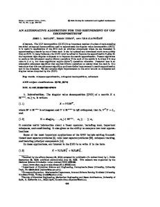
where a, b, c, and d are parameters whose values are taken to be 0.25, 3.0, 0.05, and 0.5, respectively, for our computations. For all the systems, we have used a variable step-size Runge-Kutta routine 共RKQC兲 for integration with an error tolerance ⑀ ⬃10⫺6 – 10⫺8 . All the computations were performed on a DEC Alpha based workstation running OpenVMS. We also noted the CPU time taken for each case with either of the algorithms. This is the actual time taken by the CPU to accomplish a specific process 共independent of the other processes running in the system兲. The details of the comparison between the two methods are summarized in Table I. It may be noticed that the two methods yield essentially the same Lyapunov spectrum. For any dynamical system, one of the Lyapunov exponents has to be zero 共corresponding to the difference vector ␦ z lying along the trajectory itself兲. For the Lorenz system, the Ro¨ssler hyperchaos system 共both dissipative兲, and the coupled quartic oscillators, this condition is satisfied by both algorithms. For the driven Van der Pol oscillator and the anisotropic Kepler problem, both methods fail the test. This aspect needs to be studied further. For the coupled quartic oscillators, all the exponents should be zero corresponding to the integrable case of ␣ ⫽6. This is indeed satisfied by both algorithms. In Fig. 1 we give plots of Lyapunov exponents as functions of time for a typical case. Again, there is little difference between the two algorithms as far as the convergence of the Lyapunov exponents is concerned. However, for the system of coupled quartic oscillators, the CPU time is abnormally high for the new method, corresponding to the nonintegrable case of ␣ ⫽8. This is true for both small and large energies. For large energies (⬃25 000), since the energy varied by ⬃15 when we used
RAPID COMMUNICATIONS
R1128
K. RAMASUBRAMANIAN AND M. S. SRIRAM
PRE 60
TABLE I. Comparison of the two methods for some systems with n⫽2, 3, and 4. The values given in parentheses correspond to the standard method.
System Driven van der Pol Oscillator (n⫽2)
Initial condition z 1 ⫽⫺1.0 z 2 ⫽1.0
Lorenz system (n⫽3)
z 1 ⫽0.0 z 2 ⫽1.0 z 3 ⫽0.0
Anisotropic Kepler problem (n⫽4)
z 1 ⫽1.0 z 2 ⫽2.0 z 3 ⫽1.0 z 4 ⫽0.5
Ro¨ssler hyperchaos (n⫽4)
z 1 ⫽⫺20.0 z 2 ⫽0.0 z 3 ⫽0.0 z 4 ⫽15.0
Coupled quartic oscr. (n⫽4, ␣ ⫽6)
z 1 ⫽0.8 z 2 ⫽0.5 z 3 ⫽1.0 z 4 ⫽1.3
Coupled quartic oscr. (n⫽4, ␣ ⫽8)
z 1 ⫽0.8 z 2 ⫽0.5 z 3 ⫽1.0 z 4 ⫽1.3
Lyapunov spectrum, sum (s), and CPU time (t) in sec 0.0981 共0.0987兲 ⫺6.8400 (⫺6.8411) s⫽⫺6.7419 (⫺6.7424) t⫽519.22 共825.56兲 0.9056 共0.9051兲 0.0000 共0.0000兲 ⫺14.5723 (⫺14.5718) s⫽⫺13.6667 (⫺13.6667) t⫽2394.30 共1668.68兲 0.1360 共0.1332兲 0.0831 共0.0832兲 ⫺0.0833 (⫺0.0833) ⫺0.1357 (⫺0.1331) s⫽⫺0.0000 (⫺0.0000) t⫽350.18 共201.04兲 0.1128 共0.1121兲 0.0214 共0.0196兲 ⫺0.0000 (⫺0.0000) ⫺24.7527 (⫺25.1886) s⫽⫺24.6185 (⫺25.0568) t⫽1527.58 共5594.99兲 0.0001 共0.0001兲 0.0001 共0.0001兲 ⫺0.0001 (⫺0.0001) ⫺0.0001 (⫺0.0001) s⫽0.0000 共0.0000兲 t⫽803.49 共492.09兲 0.1806 共0.1738兲 0.0001 共0.0001兲 ⫺0.0001 (⫺0.0001) ⫺0.1806 (⫺0.1738) s⫽0.0000 共0.0000兲 t⫽39012.77 共855.64兲
the RKQC routine, we also used a symplectic procedure that eliminates secular variations in the energy. With this routine, the CPU times were nearly the same for both methods. However, the new method yields poor results for the Lyapunov spectrum. For instance, corresponding to the initial condition z 1 ⫽7.0, z 2 ⫽7.0, z 3 ⫽5.0, and z 4 ⫽4.0, the Lyapunov spectra computed using the new and the standard methods are 共1.5506, 0.3254, ⫺0.3261, ⫺1.5499) and 共1.5205, 0.0001, ⫺0.0001, ⫺1.5205), respectively. We also compared the new method with another procedure for computing Lyapunov spectra with continuous Gram-Schmidt orthonormalization 关10兴. Here the number of equations that need to be integrated to obtain the complete spectrum is n(n⫹2), as compared to n(n⫹1) equations in the standard method and n(n⫹3)/2 equations in the new method, where n is the order of the system. The CPU time for this method, corresponding to the initial conditions given in Table I for ␣ ⫽8, is 7658.57 s, as compared to 39 012.77
FIG. 1. Plots of the Lyapunov exponent for the Ro¨ssler hyperchaos system. 共a兲 Highest exponent 1 , 共b兲 lowest exponent 4 . The thick and thin lines correspond to the new and standard algorithms, respectively.
with the new method 共with hardly any difference in the Lyapunov spectrum兲. In the standard method, as well as in Ref. 关10兴, after solving for the fiducial trajectory, the equations for the tangent flow are linearized equations. In the new method, these equations are replaced by the equations for the angles determining the principal axes or the bases associated with the Lyapunov spectrum and the Lyapunov exponents. These equations involving sines and cosines of the angles are highly nonlinear. For dissipative systems this nonlinearity does not pose a problem. However, in many cases, this nonlinearity renders the new method less efficient, and can even lead to inaccuracies in strongly chaotic situations. III. CONCLUSIONS
In a recently proposed new method for the computation of Lyapunov exponents, the Lyapunov exponents are calculated directly, so to say, by utilizing representations of orthogonal matrices applied to the tangent map. Since it does not require renormalization or reorthogonalization and requires a lesser number of equations, it has been claimed that it has several advantages over existing methods. To test this claim, we have computed the full Lyapunov spectrum of some typical nonlinear systems with two, three, and four variables and made a detailed comparison with the results obtained using a standard algorithm. For dissipative systems, there is reasonable agreement between the spectra obtained using the two algorithms. The CPU time taken for the computation is also comparable. However, in certain strongly chaotic situations, the new algorithm could lead to inaccuracies in the
RAPID COMMUNICATIONS
PRE 60
ALTERNATIVE ALGORITHM FOR THE COMPUTATION . . .
R1129
Lyapunov spectrum, when one uses fixed step-size integrator routines, however small the step size may be. This could be remedied by a variable step-size routine with a reasonable value of error tolerance. But this makes the new method far less efficient 共taking abnormally long times for computation兲, compared to the standard algorithm. This could be attributed to the highly nonlinear nature of the evolution equations for the tangent map inherent in this method. However,
the proposed new method is still useful as an alternate algorithm for the computation of Lyapunov spectra.
One of the authors 共K.R.兲 thanks the Council for Scientific and Industrial Research, India for financial support.
关1兴 G. Benettin, L. Galgani, A. Giorgilli, and J. M. Strelcyn, Meccanica 15, 9 共1980兲; I. Shimada and T. Nagashima, Prog. Theor. Phys. 61, 1605 共1979兲. 关2兴 A. Wolf, J. B. Swift, H. L. Swinney, and J. A. Vastano, Physica D 16, 285 共1985兲. 关3兴 G. Rangarajan, S. Habib, and R. D. Ryne, Phys. Rev. Lett. 80, 3747 共1998兲. 关4兴 G. H. Golub and C. F. Van Loan, Matrix Computations, 3rd ed. 共John Hopkins University Press, Baltimore, 1996兲. 关5兴 K. Geist, U. Parlitz, and W. Lauterborn, Prog. Theor. Phys. 83,
875 共1990兲. 关6兴 See, for instance, B. G. Wybourne, Classical Groups for Physicists 共Wiley, New York, 1974兲. 关7兴 M. Kuwata, A. Harada, and H. Hasegawa, J. Phys. A 23, 3227 共1990兲. 关8兴 O. E. Ro¨ssler, Phys. Lett. 71, 155 共1979兲. 关9兴 H. Yoshida, Phys. Lett. A 150, 262 共1990兲. 关10兴 I. Goldhirsch, P. L. Sulem, and S. A. Orszag, Physica D 27, 311 共1987兲; F. Christiansen and H. H. Rugh, Nonlinearity 10, 1063 共1997兲.
ACKNOWLEDGMENT