Missing:
Alternative Methods for Counting Overlapping Grains in Digital Images Andr´e R.S. Mar¸cal Faculdade de Ciˆencias, Universidade do Porto DMA, Rua do Campo Alegre, 687, 4169-007 Porto, Portugal
Abstract. Standard granulometry methods are used to count the number of disjoint grains in digital images. For the case of overlapping grains, the standard method is not effective. Two alternative methods for counting overlapping grains in digital images are proposed. The methods are based on mathematical morphology and are suitable for grains of circular shape. The standard and overlapping methods were tested with a Monte-Carlo simulation using 32500 synthetic images with various grain sizes and quantities, as well as different levels of noise. The overall average counting error for all images tested with intermediate amount of noise (zero mean Gaussian noise with σ = 0.05) was 6.03% for the standard method, and 4.40% and 3.56% for the overlapping methods. The performance of the proposed methods was found to be much better than the standard method for images with significant overlap between grains.
1
Introduction
There is considerable interest in the development of automatic systems for the identification and counting of grains in digital images. To quantify the properties of discrete sets of objects Matheron [1] theorized the formal concept of mathematical granulometry [2], which was later applied in image analysis to both binary and continuous tone images [3]. There are various examples of applications in the literature in fields as diverse as biochemistry [2] [4] or geology [5] [6]. The standard approach is to consider disjoint or non-overlapping grains. Dougherty [7] evaluated the effect of grain overlap, but only for small overlap between grains, and mostly from a perspective of grain separation in the segmentation process. In some applications, such as the evaluation of liquid spread in water-sensitive papers (WSP), there is considerable overlap between stains (produced by fluid droplets) in the images acquired [8], as the examples in Figure 1 show. For these type of applications there is an interest in methods that can properly address the presence of overlapping grains. The purpose of this work is to present two alternatives methods for counting grains in digital images, more suitable to overlapping grains, and to evaluate them using synthetic images that simulate WSP. The manuscript is organized as follows: in section 2 the standard approach for grain counting in digital images is presented, as well as the proposed modifications to address the problem of overlapping grains, in section 3 the evaluation strategy is described, and in section 4 the results are presented and discussed. A. Campilho and M. Kamel (Eds.): ICIAR 2008, LNCS 5112, pp. 1051–1060, 2008. c Springer-Verlag Berlin Heidelberg 2008 �
1052
A.R.S. Mar¸cal
Fig. 1. Two examples of water sensitive papers with considerable stain overlap
2
Methods
The proposed methods for counting overlapping grains use the elementary morphological operators dilation (⊕) and erosion (�). Both operators use a structuring element E, which is usually of much smaller size than the image I. The dilation of I by E is I⊕E and the erosion of I by E is I�E [9]. The morphological operator opening (◦) of I by E is defined as an erosion followed by a dilation: I ◦ E = (I � E) ⊕ E. Alternatively, the morphological operator closing (•) of I by E is defined as a dilation followed by an erosion: I • E = (I ⊕ E) � E [10]. Another morphologic operation used here is the assignment of labels to connected objects in a binary image, fn (I), where n is the number of pixel neighbors considered [11]. This procedure produces an image of the same size as the input binary image (I) where each non-null pixel of I is assigned a value according to the object number it belongs. The maximum pixel value of fn (I) is Ω(fn (I)), which corresponds to the number of n-connected objects in I. The MATLAB implementation of this procedure was used with a neighborhood of 4 pixels (n = 4) [12]. 2.1
Standard Approach for Disjoint or Non-overlapping Grains
Morphological granulometries are performed by opening an image with increasing structuring elements in order to successively diminish the image [13]. During granulometry, the image is successively sieved with a family of disks of increasing diameters [2]. The process produces images Ii = I◦Ei , where the structuring element Ei is a disk or radius i. The difference in area of the resulting images Ii+1 and Ii indicates the decrease in isolated objects of a similar size to the structuring element Ei . The estimate of the number of circular objects of radius i (NiST ) present in I is thus computed by (1), where A is the operator that computes the area of a binary image (number of pixels with value 1, ON). NiST = (A(I ◦ Ei ) − A(I ◦ Ei+1 ))/A(Ei )
(1)
Alternative Methods for Counting Overlapping Grains in Digital Images
2.2
1053
Modifications for the Overlapping Case
Instead of counting the decrease in area after each opening operation, two alternative approaches are proposed. The morphologic operation erosion is applied to the original image I, for each disk of radius i, resulting in an image I�Ei . The image label f4 (I�Ei ) is then computed for the eroded image. The first estimate of the number of circular objects of radius i (NiI ) is computed using (2). This is simply the difference in the number of 4-connected objects in the binary images produced by the erosion operator with structuring elements Ei and Ei+1 . The second estimate (NiII ) counts the number of objects that were eliminated in each iteration, using (3), where * is the image multiplication operator.
2.3
NiI = Ω(f4 (I � Ei )) − Ω(f4 (I � Ei+1 ))
(2)
NiII = Ω(f4 (I � Ei )) − Ω(f4 (I � Ei ) ∗ (I � Ei+1 ))
(3)
Example for the Standard and Overlapping Methods
Three test images were produced to illustrate the performance of the grain counting methods under well controlled conditions. These are binary images of 550 by 550 pixels, with single sized grains and with various amount of overlap between grains. The first image (Figure 2, left) has 100 grains of 20 pixel radius (R). The horizontal distance (D) between neighboring grain pairs are 50, 40, 30, 20 and 10, while the vertical distance between neighboring grains is fixed at 50. This results in 20 independent grains (no overlap, D > 2R), 20 grains in tangent pairs (D = 2R), 20 grains in pairs with low overlap (92.8% of the area retained, D/R = 3/2), 20 grains in pairs with mid overlap (80.5% of the area retained, D = R) and 20 grains in pairs with high overlap (65.8% of the area retained, D/R = 1/2). For the extreme case of full overlap (D = R) only 50% of the area would be retained and it would become impossible to distinguish the pair from a single grain. The results of the 3 counting methods applied to this image were: NiST = 88, NiI = 100, NiII = 100. The second image (Figure 2, center) has 180 grains with R = 12, and the third test image (Figure 2, right) has 216 grains with R = 10. The grains in these images are also grouped in pairs, but with the pair axes aligned in 9 different directions. The results provided by the three counting methods for the second image were NiST = 152 (-15.6% than expected) and NiI = NiII = 182 (+1.1%), and for the third image NiST = 185 (-14.3%) and NiI = NiII = 228 (+5.6%). The standard method clearly fails in the identification of the number of grains, particularly when there is a large overlap between grains. The method is based in the computation of lost area between iterations, which is effective for nonoverlapping grains, but when grains overlap, there is a decrease in overall area covered that results in an incorrect evaluation of the number of grains and their sizes. The two alternative methods proposed performed perfectly for test
1054
A.R.S. Mar¸cal
Fig. 2. Test images with 100 grains of radius 20 (left) 180 grains of radius 12 (center) and 216 grains of radius 10 (right)
image 1, but overestimated the number of grains in the other two test images. However, the estimates provided by the two overlapping methods proposed are much closer to the actual number of grains in these images than the estimates of the standard method. The additional degree of freedom introduced by allowing overlap between grains results in an increased difficulty for the counting process. In an extreme case, when grains are totally covered by others, it shall be impossible to identify their presence. However, for less extreme cases it is possible to separate and count individual grains, even when with considerable overlap between grains, as the three examples presented show.
3
Test Using Synthetic Images
A Monte-Carlo simulation was carried out to evaluate the performance of the three counting methods to identify and count overlapping grains in digital images. 3.1
Synthetic Binary Images with Overlapping Grains
Synthetic binary images were generated with N grains of radius R placed randomly in blank images of 1000 by 1000 pixels. Figure 3 shows three examples of the synthetic binary images produced: with N = 200 and R = 10 (left), with N = 400 and R = 10 (center), and with N = 400 and R = 15 (right). These examples illustrate how the overlap between grains tends to increase with N and R, thus reducing the possibilities for discrimination between grains. 3.2
Synthetic RGB Images with Overlapping Grains
To better simulate the conditions of real WSP images [8], RGB versions of the synthetic binary images were also created. Two RGB reference images of 1000 by 1000 pixels were initially produced - one using a blank WSP (RGB-blank) and
Alternative Methods for Counting Overlapping Grains in Digital Images
1055
Fig. 3. Examples of synthetic images with N grains of radius R: N = 200 and R = 10 (left), N = 400 and R = 10 (center) and N = 400 and R = 15 (right)
another using manually selected areas of WSP that were exposed to moisture (RGB-covered). These two reference signatures are very different, as a blank WSP is yellow (average RGB 241/246/56) and the WSP exposed to moisture turns blue (average RGB 71/55/210). The first step for the production of a RGB image that simulates a WSP is to produce a binary image with N grains (stains in a WSP) of radius R. This image is multiplied by the reference image RGB-covered and its complement multiplied by the reference image RGB-blank. The sum of the two multiplication results is a first version of a synthetic WSP image with N stains (grains) of radius R. Zero mean Gaussian noise with standard deviation σ is then added to each channel of the RGB image. Figure 4 shows an example of a RGB image produced by this method with N = 200 and R = 10: binary image (left), RGB without noise (center) and RGB with zero mean Gaussian noise with σ = 0.15 (right). The images presented in Figure 4 are originally in color (except for the binary image on the left), with the light gray tones corresponding to yellow and the darker areas to blue.
Fig. 4. Binary image (left) with R = 15 and N = 400 and resulting RGB images, without noise (center) and with zero mean Gaussian noise with σ = 0.15 (right)
1056
3.3
A.R.S. Mar¸cal
Experimental Procedure
A range of values were selected for N , R and σ. The number of different values used were: 10 for N (50,100,...,500), 13 for R (3 to 15), and 5 for σ (0.01, 0.05, 0.08, 0.10, 0.15). The number of images produced for each triplet (N ,R,σ) was 50, thus resulting in a total of 32500 synthetic images (10 × 13 × 5 × 50). Each RGB synthetic image was converted to binary format by color segmentation based on the Euclidean distance, using the typical RGB signature of the WSP background as reference.
4
Results
The three counting methods were applied to each of the synthetic images produced. The number of grains was computed as a function of radius, and the maximum value was used to determine the grain radius and number. The correct identification of the grain radii was achieved for every single image for methods I and II but not for the standard method that often failed for images with small sized grains. In particular, for R = 3 the standard method failed to recognize the grain size in almost all images. The error d is computed by comparing the number of grains counted (N C ) with the number of grains generated (N ), according to (4). The average error < d > is calculated as the average of d over the 50 images tested. The relative error is � = d/N and the average relative error < � >, simply referred here as counting error, is obtained by (5). � � d = �N C − N �
(4)
< � >=< d > /N
(5)
The counting error (< � >) for all pairs of N and R values tested are presented for the standard method (Table 1) and the overlaping methods I (Table 2) and II (Table 3), all using Gaussian noise with σ = 0.05. The counting error is generally quite low for all three methods, below 2-3%, for images with low values of R and N . As the values of N and R increase, the counting errors become larger. This is consistently observed both going through lines (fixed R) and columns (fixed N ) in Tables 1, 2 and 3. This is an expected result, as the amount of overlap between grains increases both with N and R. For images with high values of N and R there is considerable overlap between grains. For example, with the image size used (1000x1000 pixels), 500 non-overlapping grains of radius 15 would cover 35.5% of the image area, assuming that the grains would not touch the image edges. However, in reality the average amount of area covered by these images (N = 500 and R = 15) is only 29.5%, which is about 17% less than the maximum possible area covered. The number of separated objects is also much reduced - on average only 224.9 instead of 500 for the non-overlapping case. The overall average counting error for all images tested with σ = 0.05 (Tables 1-3) is 6.03% for the standard method, 4.40% for the overlapping method I and
Alternative Methods for Counting Overlapping Grains in Digital Images
1057
Table 1. Counting error (< � >) for the standard method (for images of N grains of radius R), with σ = 0.05 R N 3 4 5 6 7 8 9 10 11 12 13 14 15
50 fail 1.5% 3.5% 1.2% 1.3% 1.6% 2.0% 1.5% 2.0% 2.9% 2.7% 3.0% 3.6%
100 fail 1.3% 2.3% 1.1% 1.3% 1.7% 1.8% 2.1% 3.3% 3.8% 4.0% 4.6% 5.6%
150 fail 1.4% 1.9% 1.0% 1.5% 1.7% 2.0% 3.0% 4.3% 4.5% 5.1% 6.8% 7.5%
200 fail 1.1% 1.7% 0.7% 1.8% 1.8% 2.9% 3.6% 5.2% 6.5% 6.5% 8.8% 10.6%
250 fail 1.1% 1.6% 1.2% 1.9% 2.5% 3.3% 4.7% 6.3% 8.1% 8.4% 11.2% 12.8%
300 fail 1.1% 1.5% 1.2% 2.3% 2.7% 3.5% 5.4% 7.6% 9.2% 10.8% 13.2% 15.6%
350 fail 1.1% 1.7% 1.2% 2.7% 3.3% 4.5% 6.7% 9.0% 11.3% 12.5% 15.8% 19.5%
400 fail 1.3% 1.5% 1.5% 2.8% 3.7% 5.3% 7.3% 10.4% 12.6% 14.3% 18.4% 21.9%
450 fail 1.4% 1.5% 1.7% 3.1% 4.0% 5.8% 8.4% 12.2% 14.5% 16.6% 21.7% 24.9%
500 fail 1.2% 1.6% 1.8% 3.5% 4.5% 6.5% 9.2% 13.6% 16.4% 18.8% 24.1% 28.2%
Table 2. Counting error for the overlapping method I (for images of N grains of radius R), with σ = 0.05 R N 3 4 5 6 7 8 9 10 11 12 13 14 15
50 0.9% 1.3% 1.8% 1.6% 1.3% 2.0% 2.2% 1.9% 1.9% 2.5% 2.5% 2.4% 2.4%
100 1.2% 1.3% 1.9% 1.8% 1.5% 2.3% 2.6% 2.2% 2.1% 2.1% 2.7% 3.2% 2.7%
150 1.2% 0.9% 1.6% 1.6% 2.0% 1.6% 2.5% 2.8% 2.4% 2.3% 3.3% 3.8% 3.7%
200 1.2% 1.4% 1.8% 1.4% 2.2% 2.0% 3.0% 2.7% 2.6% 3.4% 3.5% 3.7% 4.9%
250 1.5% 1.4% 1.8% 2.0% 2.3% 2.5% 2.9% 3.4% 2.6% 4.3% 5.2% 7.4% 5.9%
300 2.0% 1.6% 2.1% 2.2% 2.5% 2.7% 3.6% 3.6% 3.7% 4.3% 6.7% 7.6% 8.1%
350 1.7% 1.7% 2.3% 2.5% 2.9% 3.6% 4.6% 4.3% 4.2% 5.2% 8.5% 10.4% 11.6%
400 1.9% 2.2% 2.9% 2.8% 3.2% 3.4% 5.2% 5.1% 5.4% 7.0% 10.3% 13.5% 13.9%
450 2.0% 2.2% 2.8% 3.2% 3.5% 3.6% 5.8% 6.0% 7.3% 8.8% 12.5% 16.1% 17.3%
500 2.0% 2.2% 3.4% 3.0% 3.8% 4.1% 6.2% 6.7% 7.8% 9.9% 14.9% 18.4% 19.6%
3.56% for the overlapping method II. These are averages of up to 6000 images (12 × 10 × 50), as the images with R = 3 were not considered because the standard method failed for those images. For small sized grains the performance of the standard method is slightly better than the overlapping method I, and about the same as method II. However, for larger values of R, both overlapping methods outperform the standard method. For example, for the most difficult case (N = 500 and R = 15), the counting errors are: 28.2% (ST), 19.6% (I) 14.9% (II). Comparing the two overlapping methods, it can be verified that method II performs better (or equally) than method I for all values of R and N , with a much better performance in the most difficult cases, where there is more overlap between grains.
1058
A.R.S. Mar¸cal
Table 3. Counting error for the overlapping method II (for images of N grains of radius R), with σ = 0.05 R N 3 4 5 6 7 8 9 10 11 12 13 14 15
50 0.9% 1.3% 1.8% 1.6% 1.2% 2.0% 2.2% 1.8% 1.8% 2.2% 2.4% 2.3% 2.3%
100 1.2% 1.3% 1.9% 1.7% 1.4% 2.2% 2.3% 2.2% 2.0% 1.9% 2.4% 2.6% 2.5%
150 1.2% 0.9% 1.6% 1.6% 1.8% 1.5% 2.3% 2.5% 2.1% 1.8% 2.7% 3.0% 3.0%
200 1.2% 1.4% 1.8% 1.4% 2.0% 1.9% 2.7% 2.5% 2.2% 2.4% 3.1% 2.8% 3.9%
250 1.5% 1.3% 1.8% 1.9% 2.1% 2.3% 2.4% 3.1% 2.2% 3.1% 4.3% 5.2% 4.6%
300 2.0% 1.6% 2.1% 2.1% 2.2% 2.6% 3.0% 3.1% 3.0% 3.2% 5.2% 5.3% 6.2%
350 1.7% 1.7% 2.3% 2.3% 2.5% 3.2% 3.6% 3.6% 3.2% 3.5% 6.5% 7.4% 8.6%
400 1.9% 2.1% 2.9% 2.6% 2.7% 3.1% 4.1% 4.4% 4.0% 4.7% 8.2% 9.2% 10.5%
450 2.0% 2.2% 2.7% 2.9% 3.0% 3.1% 4.5% 5.1% 5.4% 6.1% 9.7% 11.4% 13.1%
500 2.0% 2.2% 3.3% 2.8% 3.1% 3.6% 4.9% 5.5% 5.8% 6.9% 11.4% 12.8% 14.9%
Fig. 5. Counting error for images of type I with R = 10 (left) and N = 250 (right)
The results presented in Tables 1-3 correspond only to the synthetic images produced with σ = 0.05 Gaussian noise. The results for the images with other values of σ follow a similar pattern, but the counting error naturally tends to increase with σ. As an illustration, Figure 5 shows a plot with the counting error (< � >) for the overlapping method II on images with R = 10. The error is reasonably low for levels of noise 0.02, 0.05, and 0.08, increasing considerably for σ = 0.10 and even more for σ = 0.15. For those images with the highest level
Alternative Methods for Counting Overlapping Grains in Digital Images
1059
of noise (σ = 0.15) this seems to be the dominant factor, as the counting error remains almost unchanged for all values of N .
5
Conclusions
Two alternative methods were proposed for counting overlapping grains in digital images. The standard and the two overlapping methods proposed were tested with a total of 32500 synthetic images produced with randomly placed circular grains of fixed size. The overlapping methods were successful in determining the grain size in all images tested, unlike the standard method that often failed to do so for images with small sized grains. All three methods provide reasonable estimates of the number of grains present in the image, when the number and size of grains is low. As the size and number of grains increases, the overlap between grains become more frequent, which results in a larger counting error. This is particularly true for the standard method that performs much worse than the proposed overlapping methods in these situations. Overall, the proposed overlapping method II performs best, followed by the overlapping method I. The overall average counting error for all images tested with intermediate amount of noise (zero mean Gaussian noise with σ = 0.05) was 6.03% for the standard method, 4.40% for the overlapping method I and 3.56% for the overlapping method II. The results with synthetic images are very encouraging, and the proposed methods seems to be viable tools for the identification and counting of overlapping grains of circular shape in digital images.
References 1. Matheron, G.: Random sets and integral geometry. Wiley, Chichester (1975) 2. Prodanov, D., Heeroma, J., Marani, E.: Automatic morphometry of synaptic boutons of cultured cells using granulometric analysis of digital images. Journal of Neuroscience Methods 151, 168–177 (2006) 3. Serra, J.: Image analysis and mathematical morphology. Academic Press, London (1982) 4. Theera-Umpon, N., Dougherty, E.R., Gader, P.D.: Non-homothetic granulometric mixing theory with application to blood cell counting. Pattern Recognition 34, 2547–2560 (2001) 5. Francus, P.: An image-analysis technique to measure grain-size variation in thin sections of soft clastic sediments. Sedimentary Geology 121, 289–298 (1998) 6. Selmaoui, N., Repetti, B., Laporte-Magoni, C., Allenbach, M.: Coupled strata and granulometry detection on indurated cores by gray-level image analysis. Geo-Mar Lett. 24, 241–251 (2004) 7. Dougherty, E.R., Cuciurean-Zapan, C.: Optimal reconstructive z-openings for disjoint and statistically modeled nondisjoint grains. Signal Processing 56, 45–58 (1997) 8. Syngenta. Water-sensitive paper for monitoring spray distributions. CH-4002. Basle, Switzerland, Syngenta Crop Protection AG (2002) 9. Gonzalez, R.C., Woods, R.E.: Digital Image Processing. Prentice-Hall, Englewood Cliffs (2002)
1060
A.R.S. Mar¸cal
10. Gonzalez, R.C., Woods, R.E., Eddins, S.L.: Digital Image Processing using MATLAB. Prentice-Hall, Englewood Cliffs (2004) 11. Haralick, R.M., Shapiro, L.G.: Computer and Robot Vision, vol. I, pp. 28–48. Addison-Wesley, Reading (1992) 12. Using Matlab, Version 6.5. The MathWorks, Inc. Natick. MA (2002) 13. Dougherty, E.R., Sand, F.: Representation of Linear Granulometric Moments for Deterministic and Random Binary Euclidean Images. Journal of Visual Communication and Image Representation 6, 69–79 (1995)