This paper presents an algorithm used for selecting an aircraft's optimal altitude for a constant speed, level flight, cruise segment of a given length, in the ...
Altitude Optimization Algorithm for Cruise, Constant Speed, Level Flight Segment B.D. Dancila(a), R.M. Botez(a), D. Labour(b) (a) Ecole de technologie superieure, Montreal QC, (b) CMC Electronics-Easterline, Montreal QC
Abstract This paper presents an algorithm used for selecting an aircraft’s optimal altitude for a constant speed, level flight, cruise segment of a given length, in the presence of winds. This algorithm is developed for normal flight conditions, and does not consider the costs associated with the initial and final changes of altitude. The optimization criteria correspond to the minimization of the total costs, and fuel consumption, associated with flying the cruise segment. The fuel burn computing algorithm creates, for a speed schedule (a pair of Mach and IAS speed values) and standard temperature deviation (ISA_Dev), a look-up table showing the relationship between the aircraft’s altitude, gross weight at the segment start point, the travel time and the final gross weight, thus the burned fuel quantity. The algorithm’s input aircraft, navigation and atmosphere parameters are: the fuel weight and aircraft zero-fuel weight, zero fuel weight center of gravity position, the optimization distance, the cruise altitude range, the cruise speed schedule, the standard temperature deviation, segment heading, wind conditions, and the Cost Index value – representing the non-fuel operational costs, expressed in kilograms of fuel per minute. The aircraft performances and capabilities data are modeled by interpolation tables. The output parameters are represented by the optimal altitude and the corresponding quantity of fuel burned. The algorithm determines the actual range of possible cruise altitudes, corresponding to the aircraft’s configuration at the segment start point. It then determines the travel time, and the corresponding fuelburn, at each altitude. Finally, the total costs corresponding to each altitude are computed and the altitude presenting the minimal costs and fuel-burn is selected.
Introduction The optimal flight trajectory prediction is an important component in achieving current and future standards of economic efficiency, and environmental protection, adopted by the aviation industry. For the cruise phase, a modern flight management system (FMS) may be required to use one of a number of optimization strategies, which may include: the determination of the optimal speed for a given cruise altitude, the optimal altitude for a given speed schedule and cruise distance, or a complete cruise altitude profile that minimizes the flight costs [6]. The algorithm presented in this paper addresses the determination of the optimal altitude for flying a segment, characterized by its distance, heading and wind conditions, at a selected speed schedule and cost index. The optimization algorithm, developed in 1
MATLAB, was applied on an aircraft performance description model that considers the center of gravity position, which presents a more accurate, complex, and computing intensive, fuel flow to fuel-burn conversion algorithm. The optimal altitude and fuel burn predictions were compared with the data produced by a FMS, for the same aircraft model and flight conditions as those considered for the algorithm. Costs The total costs associated with flying an aircraft are determined by the sum of two factors [6]: Fuel costs (FC) – as a function of aircraft’s performances, flying conditions and flight duration Non-fuel operational costs (NFC) – proportional to the amount of time required to fly the route
Ctot = FC + NFC
(1)
Fuel costs, for constant speed level flight segments, are calculated as a continuous summation (integral) of the instantaneous fuel flow (the fuel burn rate - FBR) over the entire duration of the flight segment [6]. T flight
FC = FUELprice *
FBR t dt
0
(2)
Non-fuel operational costs are calculated using a Cost Index (CI) – a constant parameter whose value is selected according to airline’s operational policies – expressed as a rapport between the non-fuel operational costs per minute of flight, and unitary fuel price (one minute of flight equals CI kg. of fuel)[5][6]. Its expression is:
NFC = FUELprice * 60* CI * T flight
(3)
The resulting equation for the total costs can be written as [6]:
Ctot = FUELprice
T flight * 60* CI * T flight + FBR t dt 0
(4)
Expressing the total costs only in terms of kilograms of fuel, equation (4) becomes [6]: T flight
Ctot = 60* CI * T flight +
0
FBR t dt (5)
Equation (5) shows that the computation of the total cost, for an aircraft flying a segment of a given length, at a constant speed, and at a constant altitude, is composed of two independent computations: The time required to fly the segment distance. 2
The fuel burn corresponding to a given period of time. Flight segment’s travel time (Tflight)
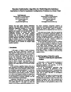
The time required to fly a given segment depends on the segment’s length, and aircraft’s ground speed. The ground speed is computed based on the aircraft’ selected speed schedule, altitude, segment heading and wind conditions [4]. Depending on the chosen wind model, we distinguish three ground speed calculation scenarios: Still air In still air, and at a given altitude, the ground speed value is constant, and equal to aircraft’s true air speed (TAS). It is not influenced by the segment heading. At each altitude, the value of the TAS is computed based on the tables describing the standard atmosphere parameters [2]. As illustrated in the Figure 1, below, the TAS presents a maximum at the crossover altitude (defined as the altitude at which the TAS, corresponding to the selected IAS schedule, equals the TAS corresponding to the selected Mach schedule) – identified in the figures as the inflexion points. Below the crossover altitude, the TAS corresponds to the IAS schedule. Over the crossover altitude, the TAS corresponds to the Mach schedule.
Figure 1 – TAS variation with the altitude, for a set of speed schedules By consequence, as illustrated in Figure 2, the segment’s travel time presents a minimum, at the crossover altitude.
Figure 2 – Travel time variation with the altitude, for a set of speed schedules 3
Constant wind Constant wind refers to the fact that, at any given altitude, the predicted wind speed and direction are constant along the flight segment. Modern FMS equipment can associate, to any waypoint in the flight plan, a table for the predicted wind speed and direction, at up to four altitudes [6]. The wind speed and direction, for a given segment and altitude, is computed through linear interpolation using the wind prediction table associated with the segment’ starting waypoint. The predicted ground speed is computed based on aircraft’s TAS, segment heading, wind speed and direction, using the “Wind Triangle Algorithm” [4]. As the predicted wind speed and direction, and aircraft’s TAS are constant, the predicted ground speed remains constant along the flight segment, at the considered altitude. Consequently, the wind layers, in the constant wind model, for a given speed schedule, have the effect of distorting the values and shapes of the variation with the altitude, of the ground speed and travel time, computed for the still air scenarios (see Figure 3 and Figure 4).
Figure 3 – Ground Speed variation with altitude, for still air and in the presence of wind (segment heading: 0deg, speed schedule: 0.78/280, wind structure: 15000/50/190; 25000/90/120; 33000/40/310)
Figure 4 – Travel Time variation with altitude, for still air and in the presence of wind (segment heading: 0deg, speed schedule: 0.78/280, wind structure: 15000/50/190; 25000/90/120; 33000/40/310) 4
Variable wind Variable wind scenarios show situations in which the predicted wind speed and direction change with the altitude and with the position along the flight segment, a correction algorithm is used to adjust the predicted value (function of the wind speed, and direction, measured at aircraft’s location), or a combination of both. It ensues that, for any given altitude, the ground speed varies along the segment’s length. The effects of the winds, in this case, are translated into an average ground speed corresponding to the segment’s travel time. Therefore, the wind influence can be regarded as distortion of the (average) ground speed and travel time, with respect to the still air conditions. For any given altitude, wind speed and direction variation along the flight segment entails a variation of the ground speed along the same flight segment. Therefore, an accurate estimation of the time required to fly the segment distance demands integrating the inverse of the ground speed, with respect to the distance, along the segment length. d
dx 0 GND _ SPEED(TAS (SpdSched, alt ), θsegm , Wind (alt , x))
Tflight
(6)
The fuel burn The cruise, constant speed, level flight, fuel-related computations currently implemented in the Flight Management System’ software are based upon aircraft’s performances and capabilities, described by one or more linear interpolation tables. The number of tables, and parameters that define each table, depend on the aircraft modeling. The list of parameters include the altitude, speed (Mach or IAS), standard temperature deviation (ISA_Dev), gross weight (gw), and depending on the aircraft modeling - the center of gravity position (cg), therefore the zero fuel gross weight (zfgw), zero fuel weight center of gravity position (zfwcg), and fuel weight (fuel). The fuel burn computation algorithm, here presented, is valid for aircraft models that consider the center of gravity position. It was conceived for use in a real-time embedded environment, and it was implemented using three software modules. The three modules are further described: The first module identifies, for each parameter associated with the performance interpolation tables used by the cruise fuel burn computations, the values that delimit linearity domains in all the aforementioned interpolation tables, directly or indirectly. The second module performs, for a given speed schedule, ISA_Dev, and range of cruise altitudes, the conversion from the aircraft’s constant-speed, level-flight, cruise – fuel flow – performance representation, based on interpolation tables, to a “fuel_burn” look-up table describing the gross weight variation (i.e. the fuel burn variation) as a function of the cruise altitude and flight time. The conversion is performed upon each change of the speed schedule or ISA_Dev parameters. The table is subsequently used in all fuel burn computations associated with the optimal altitude algorithm, for the selected speed schedule and temperature deviation. The third module determines the fuel burn using the pre-computed fuel_burn table, the flying altitude, aircraft’s gross weight at the initial point of the flight segment, and the time required to fly the segment (determined based on the altitude, segment length, heading, speed schedule and wind conditions). 5
The optimal altitude The optimal altitude module determines the flying altitude yielding the minimal cost, and fuel burn, by evaluating equation (5) for each valid altitude in the range of considered cruise altitudes. It executes upon user’s request or at regular intervals of time – as configured by the FMS application. The sequence of tasks, performed by this module are: 1. Determination of the set of valid cruise altitudes to be considered for determining optimal altitude. 2. Computing the time required to fly the segment distance (Tflight(alt)), at each altitude. 3. Computing the fuel burn, function of the aircraft’s gross weight at the segment start point, and the corresponding travel time, at each altitude. 4. Computing the total cost, as described by equation (5), at each attitude. 5. Determination of the optimal altitude, yielding the minimal cost and fuel burn. Algorithm performances for “Still Air” conditions The general algorithm performances are analyzed with respect to speed/response time and accuracy. As the fuel burn modeling contribution, to the general performances of the optimal altitude algorithm, presents a special interest, we chose to eliminate possible differences, resulted from the wind modeling, by analyzing the still air flight conditions. A number of 355 test cases were investigated. Speed / Response time Given the real-time nature of the FMS software, two response times are critical: the time required to generate a fuel-burn look-up table, and the time required to determine the optimal altitude (that includes the times used for retrieving the fuel burn data from the look-up table, at each cruise altitude). The constraints imposed on each response time are different. As expected, there is a direct relationship between the fuel-burn module’s response time, the number of altitudes and the fuel burn weight span for which the table is being generated. Figure 5, below, illustrates the response times obtained on generating fuel-burn tables corresponding to 22 altitudes, and a fuel weight variation corresponding to flight times between approximately 2 and 10 hours, - ranging from 12 sec to 75 sec.. As mentioned earlier, the optimal altitude is obtained by performing a sequence of two, independent, computations: determining the travel time and computing the fuel burn corresponding to that travel time. Also, we note the fact that the travel time computation depends on the wind model adopted, and also on the particular configuration of the trajectory (number of sub-segments) and wind structure (number of wind layers). More, once the wind model is adopted, and a corresponding computing algorithm implemented, the time required to determine the travel time is the same, irrespective of the selected fuelburn and optimal altitude selection algorithms. We are interested in characterizing the optimal altitude module’s response time in a way that illustrates its performances, and those of the fuel burn algorithm, irrespective of the travel time model. Therefore, we chose not to include the travel time computation in the evaluation of the optimal altitude module’s response time. Figure 6, below, illustrates the response times of the optimal altitude module performed on segments of 500 Nm.. The response times where of up to 0.05 sec. 6
Figure 5 Intermediary module’s response time (fuel-burn table generation)
Figure 6 Optimal altitude module response time (travel time computation not included) The algorithm evaluations were conducted in a MATLAB-based environment, running on a Microsoft Windows XP Professional, 2.79 GHz, AMD Phenom(tm) II X4 Processor based computer. Accuracy We investigated two parameters related to the optimal altitude: the differences between the optimal altitudes and the fuel burns computed by the optimization algorithm, and those predicted based on the travel times and fuel burns generated by the FMS. The evaluations were conducted for the still air conditions, to allow a better characterization of the fuel burn model, and for cost index values of 0, 15, 35, 50 and 100. Figures 7 and 8 show that, for the set of configurations considered in the tests, there were differences in the predicted optimal altitude of up to 2000 ft..
7
Figure 7 – Optimal altitude prediction differences – still air conditions, CI = 0, 15, 35, 50 and 100
Figure 8 – Optimal altitude prediction difference in % – still air, CI = 0, 15, 35, 50 and 100 Differences were also noticed regarding the quantities of fuel burned predicted by the optimization algorithm, and the FMS. Figures 9, 10 and 11 illustrate the spectrum of fuel burns predicted by the optimization algorithm, as well as the absolute and relative differences with respect to the FMS data, corresponding to the set of test configurations, analyzed.
Figure 9 – Fuel Burn computed by the algorithm – still air conditions 8
Figure 10 – Fuel Burn – relative differences – still air conditions
Figure 11 – Fuel Burn – absolute differences – still air conditions Conclusions In the case of the fuel-burn look-up table generation, longer response times are acceptable as the data is generated/ updated at intervals of time determined by changes in the speed schedule or ISA_Dev parameters. Usually, these events occur at intervals of time of at least one hour [6]. More, well chosen update policies, based on maintaining valid fuel-burn data for a given flight duration, can reduce the computation volume, thus the time necessary to generating the table data. The constraints imposed on the optimal altitude’s module response time are more restrictive. They relate to the requirement to provide the pilots with timely, optimal altitude information advisory. As indicated by the test data, the algorithm’s response time - excluding the travel time computation - is in the range of 50ms. When the travel time computation is considered, the response time is increased with a period equal to the product of the number of altitudes and the time required for computing the travel time for each altitude. The differences related to the quantities of fuel burnt, estimated by the optimization algorithm and by the FMS, correspond to the differences in the fuel burn modeling. The altitude optimization algorithm presented in this paper proposes a faster, more precise, fuel burn model which follows the continuous fuel-flow variation with time, as the aircraft’s gross weight and center of gravity position change. As expected, the differences in fuel burn determine a difference between the optimal altitudes computed by the optimization algorithm, and those estimated based on the FMS data, for still air conditions. This means that, for situations considering the wind, the number of cases that lead to differences between the optimal altitude calculated by the algorithm presented in this paper, and the FMS, can increase. 9
A first advantage of the optimization algorithm is the fact that it allows, for each altitude, the estimation of the quantity of fuel burnt, in one pass, irrespective to the segment’s distance or configuration. Also, we appreciate that the algorithm provides a good trade-off between the time required to generate the fuelburn look-up tables, relative to the period of flight time for which they provide data, and the optimal altitude computation speed and accuracy. Another potential gain is the fact that the fuel-burn look-up tables may be used in subsequent constant-speed, level-flight, cruise computations of flight segments defined not only by distance, but also by duration.
Aknowledgements We would like to thank to CMC Electronics-Easterline, Mr. Rex Hygate and Mr. Claude Provencal for our collaboration opportunity. We would also like to thank Mr. Jeremy Dupont, Mr. Sidbe Souleymane and Mr. Lord Tevoedjre for their contribution to obtaining the FMS fuel burn and travel time validation data. References [1]
Federal Aviation Administration, 2007, "Aircraft Weight and Balance Handbook", Online. . Retrieved on November 10, 2010.
[2]
Asselin, M., 1997, “AIAA Education Series: An Introduction to Aircraft Performance”, Reston, Virginia, USA: American Institute of Aeronautics and Astronautics, Inc., 339 pages.
[3]
Butcher, J. C., 1987, “The numerical analysis of ordinary differential equations: Runge-Kutta and general linear methods”, New York, USA: Wiley-Interscience, 512 pages.
[4]
Botez, R., Notes de laboratoire, Introduction à l’avionique, révisée septembre 2006
[5]
Liden, S., "Practical Considerations in Optimal Flight Management Computations," American Control Conference, 1985 , vol., no., pp.675-681, 19-21 June 1985. Online. . Retrieved on May 22, 2010.
[6]
Liden, S., "Optimum cruise profiles in the presence of winds," Digital Avionics Systems Conference, 1992. Proceedings., IEEE/AIAA 11th , vol., no., pp.254-261, 5-8 Oct 1992. Online. < http://ieeexplore.ieee.org/stamp/stamp.jsp?tp=&arnumber=282147&isnumber=6983>. Retrieved on May 7, 2010.
[7]
Liden, S., "Optimum 4D guidance for long flights," Digital Avionics Systems Conference, 1992. Proceedings., IEEE/AIAA 11th , vol., no., pp.262-267, 5-8 Oct 1992. Online. > Retrieved on May 22, 2010.
10