2456
OPTICS LETTERS / Vol. 32, No. 16 / August 15, 2007
Amplitude point-spread function measurement of high-NA microscope objectives by digital holographic microscopy Florian Charrière,1,* Anca Marian,1 Tristan Colomb,2 Pierre Marquet,2 and Christian Depeursinge1 1
Ecole Polytechnique Fédérale de Lausanne (EPFL), Imaging and Applied Optics Institute, CH-1015 Lausanne, Switzerland 2 Centre de Neurosciences Psychiatriques, Département de Psychiatrie DP-CHUV, Site de Cery, CH-1008 PrillyLausanne, Switzerland *Corresponding author:
[email protected] Received June 13, 2007; accepted July 11, 2007; posted July 24, 2007 (Doc. ID 84133); published August 10, 2007
We present here a three-dimensional evaluation of the amplitude point-spread function (APSF) of a microscope objective (MO), based on a single holographic acquisition of its pupil wavefront. The aberration function is extracted from this pupil measurements and then inserted in a scalar model of diffraction, allowing one to calculate the distribution of the complex wavefront propagated around the focal point. The accuracy of the results is compared with a direct measurement of the APSF with a second holographic system located in the image plane of the MO. Measurements on a 100⫻ 1.3 NA MO are presented. © 2007 Optical Society of America OCIS codes: 090.1760, 090.1000, 110.1220, 110.4850.
The point-spread function (PSF), the image of a single source point through the optical system, remains today the usual way to characterize an optical imaging system, specifically a microscope objective (MO). Commonly, only the intensity point-spread function (IPSF) is considered, neglecting the phase point-spread function (PPSF). In phase-sensitive microscopy techniques, including digital holographic microscopy (DHM) [1], an exact knowledge of the PPSF becomes of major importance to properly interpret the measured phase signal, and eventually compensate for the aberrations in the system. Therefore, measuring both the IPSF and the PPSF, defining the complex amplitude point-spread function (APSF), is mandatory to fully characterize a MO. Interferometric techniques, requiring a three-dimensional (3D) scan of the focal region with several signal acquisitions at each position, were proposed by Selligson [2] and Juskaitis and Wilson [3]. Another idea consists in measuring the complex wavefront at the exit pupil of the MO and recovering the 3D APSF with a diffraction calculation based on these pupil-function (PF) measurements. Beverage et al. used a Shack– Hartmann wavefront sensor combined with a Fourier transform calculus to recover its PSF [4]; the PF sampling is relatively low compared with the sampling of a CCD camera, as used in the present Letter, which can limit an accurate extraction of all the PF aberrations. Török and Fu-Jen used a Twyman–Green interferometer for PF measurement and the Debye– Wolf diffraction theory to predict the complex APSF [5]; a well-calibrated spherical mirror is required as reference, and a double passage of the light through the MO may cause certain aberrations to cancel and others to double. Hanser et al. obtained the complex PF from defocused IPSF images of subresolution beads with a phase-retrieval algorithm [6]; a comparison between the recovered 3D PSF and direct measurement is presented only for the IPSF, neglect0146-9592/07/162456-3/$15.00
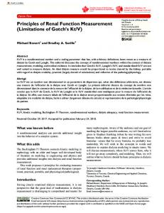
ing the PPSF. Digital holography has finally already been used in a live star test procedure by Heil et al. [7], but only IPSF was again considered. In the present Letter, a pupil-based evaluation of the 3D APSF is, for the first time to our knowledge, compared in amplitude and phase with a direct measurement of the APSF in the image plane of the MO, thanks to an original digital holographic setup involving two cameras. The setup (Fig. 1), is based on a Mach–Zehnder interferometer. The light source is a = 532 nm laser (frequency-doubled Nd:YAG) with adjustable power up to 100 mW. In the object arm, the laser is coupled in a scanning near-field optical microscopy (SNOM) fiber with a 60 nm diameter emitting tip used as a pointlike object. The MO is mounted on micrometric xyz stages with tilt facilities for a proper alignment of the MO on the optical axis. The fiber is installed on a piezoelectric xyz stage, permitting nanometric displacements within a range of 80 m. The first CCD camera, CCD1, is positioned at a distance of 1500 mm to create a sufficiently high magnification (about 1000⫻ for a 100⫻ MO) to obtain an optimal
Fig. 1. Setup for APSF measurement: BS, beam splitter; BE, beam expander, NF, neutral density filter; / 2 halfwave plate; M, mirror; FC, fiber-coupling lens; PS, piezo system, MS, micrometric stage; MO, microscope objective; O, object wave; R, reference wave. Inset, detail of the offaxis geometry at the incidence on the CCD. © 2007 Optical Society of America
August 15, 2007 / Vol. 32, No. 16 / OPTICS LETTERS
sampling by the CCD of the SNOM tip diffraction; here the CCD is used with sensitive area around 3.4 mm in size (512⫻ 512 pixels with size 6.7 m). A beam splitter, placed as close as possible from the MO, enables a second CCD camera, CCD2, to capture an image of the PF of the MO. The reference wave R is first enlarged with a beam expander, after which it is superimposed, by means of beam splitters at two different locations on the object beam O to produce a hologram on each CCD. An off-axis geometry was considered on both CCDs (see inset Fig. 1). The light intensity of the reference beam is adjusted with neutral density filters. Measurements presented here have been achieved on a vibrations-insulating table protected by curtains. The object and the reference arms were surrounded by plexiglass tubes to minimize the perturbations coming from the air turbulences. Recorded holograms are processed as follows. First, a filtering in the Fourier space is achieved to preserve only the interesting interference term while removing the DC term and the twin image term [8], after which the reillumination of the filtered hologram with the reference wave is simulated. An automatic algorithm (15 Hz with a P4 2.8 Ghz), extensively described in [9], performs this procedure, which must carefully be carried out to avoid any phase-error generation during the reconstruction process. For a given position of the SNOM tip, the processing of a single digital hologram recorded on CCD1 allows for a quantitative measurement of the transverse APSF in amplitude and phase. Thus, a single scan of the SNOM tip along the optical axis is sufficient to acquire a stack of holograms describing the complete 3D APSF of the MO. This method, described completely in [10], presents several advantages, as far as speed and ease of use are concerned (the scan is performed at 25 Hz), when compared with other techniques [2–7]. On the CCD2-hologram, the recorded object wavefront corresponds in first approximation to the MO PF. This approximation results from the very slow convergence of the beam emerging from the MO [11], which indeed forms an in-focus image on CCD1 placed at a distance of 1500 mm, much larger than the short propagation distance between the real MO
2457
pupil and the CCD2 chip (⬃50 mm). In [9] Colomb et al. explains how to compensate for the phase aberrations induced by the optical component of the setup, including the MO, in the reconstructed phase images. This compensation is based on the evaluation of the phase distribution along profiles traced in the phase image at locations where the phase is known to be constant. This automatic procedure is able to provide quantitative values of the aberrations in terms of coefficients calculated according to a mathematical model. In [9], a polynomial model was used to describe the phase function, while in the present study a Zernike polynomials (ZP) description is used. The ZP Zi are specifically well adapted to accurately describe the phase aberrations in the pupil aberration function P共x , y兲, which can be developed in a series P共x , y兲 = 兺i␣iZi, where the ␣i are coefficients and the Zi are defined on a circular pupil with unitary radius. A summary of the used Zi is presented in Table 1. To properly evaluate the aberration coefficients, the fitting procedure of [9] is applied three times sequentially. First, a simple 2D linear mathematical model is used in the reconstruction process to compensate for the tilt aberration due to the off-axis geometry. The corresponding intensity and phase distribution is presented in Figs. 2(a) and 2(b). Second, a 2D parabolic function is applied on the obtained phase distribution to compensate for the field curvature due to the focusing of the wavefront to CCD2. The remaining phase function distribution, representing the aberrations of the PF, is presented in Fig. 2(c). Third, the Zernike polynomials model is applied to the aberration function, providing its direct decomposition in terms of aberration coefficients. Figure 2(d) shows the phase distribution after subtraction of its evaluation with the Zernike polynomial, and as expected appears nearly constant, except the remaining circular patterns due to the light diffraction on MO aperture present on all the phase images of Fig. 2, proving that the used model is able to correctly describe the aberration function. The measurements presented in this Letter have been achieved with a 100 ⫻, 1.3 NA MO, in immersion oil (1.518 refractive index), but without coverslip to intentionally introduce aberrations. In Table 1, the extracted coefficients for each aberration type are presented, showing a pre-
Table 1. Zernike Polynomials and Measured Coefficients in the Pupil of the MO Polynomial Z0 Z1 Z2 Z3 Z4 Z5 Z6 Z7 Z8 Z9 Z10
Cartesian Form
Description
Coefficient
1 2x 2y 31/2共2x2 + 2y2 − 1兲 61/2共2xy兲 61/2共x2 − y2兲 1/2 8 共3x2y + 3y2 − 2y兲 81/2共3x3 + 3xy2 − 2x兲 81/2共3x2y − y3兲 81/2共x3 − 3xy2兲 1/2 4 5 共6共x + 2x2y2 + y4 − x2 − y2兲 + 1兲
Piston Tilt y Tilt y Power Astig. y Astig. x Coma y Coma x Trefoil y Trefoil x 1ary spherical
−4.930 0.051 −0.008 −0.338 0.038 0.069 0.034 −0.051 0.031 0.018 −0.573
2458
OPTICS LETTERS / Vol. 32, No. 16 / August 15, 2007
Fig. 2. Reconstructed images of the pupil hologram: (a) intensity, (b) direct measured phase, (c) aberration function, (d) residual phase after aberration function subtraction. Phase images gray-scale range is between − and .
dominant primary spherical aberration. The extracted coefficients and the corresponding aberrations were introduced in a scalar model of diffraction [12] to calculate the 3D APSF of our MO in the situation described in Fig. 3: U共r2, ,z2兲 =
i
冕 冕 2
0
␣
P共, 兲exp关ikr2 sin cos共 − 兲
0
− ikz2 cos 兴sin dd ,
共1兲
where U共r2 , , z2兲 is the APSF in polar coordinates, k is the wavevector, ␣ is the maximum angle of convergence of rays in image space, and 共 , 兲 is the pupil aberration function in term of and (see Fig. 3). Therefore, with our setup, we are able to compare the APSF calculated from a single evaluation of aberrations coefficients of the MO PF with a direct measurement of the 3D APSF in the MO image plane performed by scanning the SNOM tip along the optical axis. The results are summarized in Fig. 4, presenting x–z and x–y image comparisons in amplitude and phase between experimental APSF (top) and calculated with the scalar model of diffraction with aberration description extracted in the pupil (bottom). In the middle of Fig. 4, a completely calculated APSF obtained with the Gibson and Lanni model was added, which predicts the APSF for a use of the MO under nonstandard conditions [13]. As it can be seen on Fig. 4, the two measured APSFs and the theoretical one are in good agreement. This work illustrates
Fig. 3. Focusing through a lens of aperture a, focal f, and maximum subtended half-angle ␣.
Fig. 4. (a) x–z and (b) x–y image comparisons in amplitude and phase between APSF measurement (top) calculated APSF with the Gibson and Lanni model (middle) and calculated with the scalar model of diffraction with aberration description extracted in the pupil (bottom). Measurements performed in oil 共n = 1.518兲 without coverslip for a ⫻100 1.3 NA microscope objective. (Intensity images are enhanced by a nonlinear distribution of the gray levels; phase images gray-scale range is between − and .)
that a reliable estimation of the complete 3D APSF can be extracted from a single holographic acquisition of a MO PF. The validity of the method is for the first time to our knowledge not only attested through the comparison with a well-known theoretical aberrations model but also with a direct and quantitative measurement of the 3D APSF. The single-hologram recording, allowing one to drastically reduce the acquisition time and consequently the stability requirement, remains the main advantage of the pupil evaluation method compared with the direct measurement method. This research has been supported by the Swiss National Science Foundation grant 205320-112195/1. References 1. P. Marquet, B. Rappaz, P. J. Magistretti, E. Cuche, Y. Emery, T. Colomb, and C. Depeursinge, Opt. Lett. 30, 468 (2005). 2. J. L. Selligson, “Phase measurement in the focal region of an abberated lens,” Ph.D. dissertation (University of Rochester, 1981). 3. R. Juskaitis and T. Wilson, J. Microsc. 189, 8 (1998). 4. J. L. Beverage, R. V. Shack, and M. R. Descour, J. Microsc. 205, 61 (2002). 5. P. Török and K. Fu-Jen, Opt. Commun. 213, 97 (2002). 6. B. M. Hanser, M. G. L. Gustafsson, D. A. Agard, and J. W. Sedat, J. Microsc. 216, 32 (2004). 7. J. Heil, J. Wesner, W. Müller, and T. Sure, Appl. Opt. 42, 5073 (2003). 8. E. Cuche, P. Marquet, and C. Depeursinge, Appl. Opt. 39, 4070 (2000). 9. T. Colomb, E. Cuche, F. Charrière, J. Kühn, N. Aspert, F. Montfort, P. Marquet, and C. Depeursinge, Appl. Opt. 45, 851 (2006). 10. A. Marian, F. Charrière, T. Colomb, F. Montfort, J. Kühn, P. Marquet, and C. Depeursinge, J. Microsc. 225, 156 (2007). 11. W. Wang, A. T. Friberg, and E. Wolf, J. Opt. Soc. Am. A 12, 1947 (1995). 12. M. Gu, Advanced Optical Imaging Theory (SpringerVerlag, 2000). 13. S. F. Gibson and F. Lanni, J. Opt. Soc. Am. A 8, 1601 (1991).