An Abstract Domain Extending Difference-Bound ... - Semantic Scholar

An Abstract Domain Extending Difference-Bound Matrices with Disequality Constraints? Mathias P´eron and Nicolas Halbwachs {Mathias.Peron,Nicolas.Halbwachs}@imag.fr V´erimag?? ,

Grenoble – France

Abstract Knowing that two numerical variables always hold different values, at some point of a program, can be very useful, especially for analyzing aliases: if i 6= j, then A[i] and A[j] are not aliased, and this knowledge is of great help for many other program analyses. Surprisingly, disequalities are seldom considered in abstract interpretation, most of the proposed numerical domains being restricted to convex sets. In this paper, we propose to combine simple ordering properties with disequalities. “Difference-bounds matrices” (or DBMs) is a domain proposed by David Dill, for expressing relations of the form “x − y ≤ c” or “c1 ≤ x ≤ c2 ”. We define d DBMs (“disequalities DBM”) as conjunctions of DBMs with simple disequalities of the form “x 6= y” or “x 6= 0”. We give algorithms on d DBMs, for deciding the emptiness, computing a normal form, and performing the usual operations of an abstract domain. These algorithms have the same complexity (O(n3 ), where n is the number of variables) than those for classical DBMs, if the variables are considered to be valued in a dense set (R or Q). In the arithmetic case, the emptiness decision is NP-complete, and other operations run in O(n5 ). Keywords: abstract domains, alias analysis, difference-bound matrices, disequalities, static analysis

1

Introduction

In many situations, integer variables are used to address objects: it is the case with array indexes, memory addresses and pointers in languages like C, and — this last case being the initial motivation of this work — with the addressing of devices (memories, processors, sensors,. . . ) in systems-on-chips. It is well-known that this kind of addressing mechanism raises aliasing phenomena: these aliasing problems are error-prone, can make the programs obscure, and tremendously complicate their analysis: if i = j, then A[i] and A[j] ?

??

This work has been partially supported by the APRON project of the “ACI S´ecurit´e et Informatique” of the French Ministry of Research. Verimag is a joint laboratory of Universit´e Joseph Fourier, CNRS and INPG associated with IMAG.

are aliased, meaning that any change to A[i] implicitly changes A[j]. Knowing that i = j allows this fact to be precisely captured; knowing that i 6= j allows to keep A[j] unaffected by the changes to A[i]; ignoring whether i = j or not forces any change to A[i] or A[j] to potentially affect (i.e., lose information about) the other. So, determining whether two addresses may or must be equal is an important goal. Most abstract domains classically used to analyze the behavior of numerical variables (like affine equations [Kar76], intervals [CC76], octagons [Min01], octahedra [CC04], polyhedra [CH78]), take equalities into account, but cannot be used for determining disequalities, because they are convex . On the other hand, equality and disequality relations, considered alone, are too poor to permit an interesting analysis: the only new relations that one can deduce from a set of equalities/disequalities come from the transitivity of ’=’ ((x = y ∧ y = z) ⇒ x = z) and the obvious rule (x = y ∧ x 6= z) ⇒ y 6= z. This why it is interesting to combine this kind of relations with other properties, which enrich the deduction power: in this paper, we intend to combine equalities/disequalities with ordering relations. For instance the obvious rule (x ≤ y ≤ z ∧ x 6= y) ⇒ x 6= z may allow non completely trivial deductions. Our goal is to extend an existing domain with disequalities, without increasing the complexity of the representation and operations. In this paper, we study such an extension of the domain of difference-bounds matrices [Dil89,ACD93], used for expressing relations of the form c1 ≤ x ≤ c2 and c1 ≤ x − y ≤ c2 . The simplest kind of disequalities that we can add to these inequalities, are of the form (x − y 6= 0). It is enough for our initial goal, and, coupled with difference-bounds matrices, they allow strict inequalities to be expressed. Now, if we consider also disequalities of the form (x − y 6= c), we get systems of constraints of arbitrary size (e.g., x − y 6= 0 ∧ x − y 6= 2 ∧ x − y 6= 4 . . .) which contradicts our goal of not increasing the complexity. So, we will limit ourselves to inequalities of the form (x − y 6= 0) or (x 6= 0). The content of the paper is the following: Section 2 is a rapid review of the related works. In Section 3, we recall the definition of Difference-Bound Matrices and the main algorithms used for their manipulation, in particular the use of potential graphs. In Section 4 we define “disequalities DBM” (or d DBM), which are a simple extension of DBMs with simple disequality relations of the form (x 6= y). The notion of potential graph is extended into “disequal potential graphs”. Section 5 is devoted to the central problem of deciding emptiness of the domain of solutions of a d DBM, and of normalizing d DBMs. Two cases are distinguished, according to whether the solutions are searched in a dense numerical set (like R or Q) or in the set of integers. In the dense case, we exhibit algorithms for emptiness check and normal form computation, with the same theoretical complexity as in the case of classical DBMs. In the arithmetic case, unfortunately, the emptiness problem is NP-complete, and the complexity of the computation of a normal form increases from n3 to n5 (n being the number of variables). However, notice that the dense domain is a correct approximation of

the discrete one. Section 6 describes other classical operators on d DBMs, and Section 7 gives some simple examples of application to program analysis.

2

Related Works

Several structures for representing finite unions of convex sets have been proposed in the model-checking community. In particular, “difference decision diagrams” [MLAH99] and “clock difference diagrams” [LPWY99] are more general than the domain we consider, but with an exponential complexity. Another way of dealing with finite unions of convex set is by using “dynamic partitioning” in abstract interpretation [Bou93,JHR99,MR05,SISG06]. This could be used, for our problem, by separating the cases i < j and i > j. However, here also, this can involve an exponential partitioning. Of course, some non convex abstract domains have also been proposed, like congruences [Gra91,Mas93], but with a non comparable expressivity with our domain. The weakly relation domains proposed by [Min02] are a family of numerical domains, not necessarily convex, based on DBM alike representation and algorithmic. However, strict conditions on expressible constraints do not allow disequations. In Constraint Logic Programming (CLP), algorithms were proposed to deal with constraints on finite domains. Constraints propagation is expensive, in particular because of representation problems [HS03]. [HS97] considers a restricted class of constraints (±x ± y ≤ c), corresponding to octagons [Min01], for which they propose a polynomial solver. Disequalities are not considered, because of the NP-completeness of the satisfiability problem. However, [Pug98] notices that, if all variables are pairwise different, the satisfiability can be checked in O(n log n). In dependence analysis (which concerns alias analysis among array elements), many approaches are based on the resolution of linear constraints (e.g., [PW98] use the Omega library). Among these works, [SW02] addresses constraints of the form (±x ± y ≤ c) and disequalities. However, they use algorithmic devoted to more general constraints (Omega Test), and they don’t have the same concerns, since they don’t need to compute a normal form. About normal forms of systems of linear inequalities and disequalities, we will use Lassez’s works [LM92]. Imbert [Imb93] addresses the problem of eliminating variables from such systems. All these results are too general with respect to the constraints we consider, and only apply when solutions belong to dense sets.

3

Difference-Bound Matrices [Dil89]

Difference-Bound Matrices (DBMs) are a practical representation of potential constraints (x − y ≤ c) introduced by D. Dill [Dil89]. Let Var = {v1 , ..., vn−1 } be a finite set of variables, V (= Z, Q or R) be the numerical set in which variables and constants take their values, and V be the extension of V with +∞, ordered as usual. Let C be a set of potential constraints

(vi − vj ≤ c) where c ∈ V and vi , vj ∈Var. The DBM representing C is a n × n matrix M defined by (cf. Figure 2(a)): Mij = inf{c | (vj − vi ≤ c) ∈ C} where inf(∅) = +∞. In other words, if there is some constraint vj − vi ≤ c in C, then Mij equals (the tightest) c, otherwise it is +∞. A special variable v0 ∈ Var, always valued to zero is used to express bounds on variables: (vi ≤ c) is written (vi − v0 ≤ c). The set of all possible valuations of the variables represented by a DBM M will be called its domain, and will be noted D(M ). Potential Graph. DBMs enjoy a useful graphical representation, called potential graphs, interpreting a DBM M as the adjacency matrix of a weighted directed graph (Figure 2(b)). In the potential graph, the variable v0 corresponds to the node labelled by 0. Emptiness Test and Closure. Using the potential graph representation, we understand that unfeasible sets of constrains are only those which form a circuit with a strictly negative weight in the graph. As a consequence, in order to test whether the domain of a DBM is empty, we simply have to check for the existence of such a circuit: this could be achieved in polynomial time (O(n3 ), e.g., with Bellman-Ford algorithm). Because any potential graph including a strictly negative cycle is one possible representation of an empty domain, we are interested in finding a normal form for non-empty DBMs. Then, the shortest-path closure of their potential graph is well-defined and can be computed by the Floyd-Warshall algorithm that runs in O(n3 ) time (Figure 1). for i ← 0 to n − 1 do Mii ← 0 for k ← 0 to n − 1 do for i ← 0 to n − 1 do for j ← 0 to n − 1 do Mij ← min(Mij , Mik + Mkj ) ; Figure1. The Floyd Warshall algorithm [CLRS90] computes the shortest-path closure of a weighted digraph represented by a matrix M

Through the potential graph, the algorithm computes, for each pair of variables, the implicit constraints obtained by summation over paths of the graph, and uses the tightest one for replacement. The resulting graph represents a DBM with the same domain as the initial one, and minimal bounds for representing this domain: it is indeed a normal form. Figure 2 is an illustration of the execution of the closure algorithm of DBMs.

0 

5

3≤x≤5 −4 ≤ y ≤ 2

0 1 0 +∞ −3 4 x @ 5 +∞ 14 A y 2 +∞ +∞ (a)

4 -3 2

x

-1 9 14 (b)

y

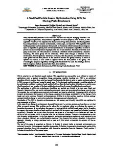
8 > 1 ≤ x, y, z ≤ 2 < x 6= y x 6= z > > : y 6= z

(a)

(b)

−1 2 2

0

y

−1

−1 2

z (c)

Figure3. (a) A set of constraints, (b) its associated d DBM and (c) its disequal potential graph

5

Emptiness Test and Normal Form

As for DBMs, we need to define a normal form, which will work for non-empty d DBMs, in order to decide equivalence of domains by a simple syntactic check, and to easily get all the consequences of given set of constraints. In this section, we provide closure algorithms to compute the normal form of a d DBM, separating the dense case (V = Q or R) and the arithmetic case (V = Z). By analogy with classical DBMs, we define the normal form M of a d DBM M by: M = infE {M 0 | D(M ) = D(M 0 )} In the arithmetic case, such normalization will narrow some bounds for arithmetic reasons: for instance the set of constraints {x 6= 0, x ≤ 0} must be replaced by {x 6= 0, x ≤ −1}. Unfortunately, this is not the only difficulties brought by arithmetic: the emptiness test problem will be in the NP-complete class [RI80].

5.1

The Dense Case

Testing Emptiness. d DBMs are extensions of DBMs by disequality constraints. Of course, the domain of a d DBM (M ≤ , M 6= ) can be empty because of the emptiness of the domain of M ≤ (which we know how to check), but it can also be empty because of the disequalities. In the case where variables take values in a dense set, the following result due to Lassez and McAloon [LM92] solves the problem, thanks to the independence of disequalities. The constraints concerned by the theorem are more general than ours, but in our special case, the result is the following: Theorem 1 (independence of disequalities (Lassez et al., 1992)). Let I be a system of linear inequalities, and D be a finite set of linear disequalities. Then the conjunction of I and D is feasible if and only if, for each single disequality d ∈ D, the conjunction of I and {d} is feasible. In other words, for a d DBM (M ≤ , M 6= ), if no single disequality eliminates all the solutions of M ≤ , there is no way for a finite number of disequalities constraints to make together the system unsatisfiable. As a consequence, in d DBMs, the only way for a disequality constraint to make the system unsatisfiable is to contradict an equality between the corresponding variables. Thus the emptiness test boils down to check, for each disequality constraint between variables, that these variables are not forced equal by the DBM component of the d DBM (Figure 4).

empty ← false ; for i ← 0 to n − 2 as long as ¬empty do for j ← i + 1 to n − 1 as long as ¬empty do 6= if Mij then ≤ ≤ empty ← Mij = 0 ∧ Mji =0 Figure4. The algorithm testing d DBM emptiness in the dense case. Runs in O(n2 ) time

This test is correct when M ≤ is in normal form: all equalities must have been expressed to perform this syntactic check. Normal Form and Closure Algorithm. In order to compute the normal form of a d DBM (M ≤ , M 6= ), we can first apply the closure of DBMs to M ≤ . This makes sense because, in the dense case, disequality constraints will not involve any narrowing of the bounds in M ≤ . Now, M 6= must be completed with all the disequalities resulting from the conjunction of M ≤ and M 6= . These inequalities are deduced according to 3 rules: 1. vi − vj ≤ c, c < 0 ⇒ vi 6= vj

2. vi = vj ∧ vj = 6 vk ⇒ vi 6= vk 3. vi ≤ vj ≤ vk ∧ vj 6= vk ⇒ vi 6= vk Rules (1) and (2) can easily be applied, in O(n3 ), using the potential graph: rule (1) says that any arc with negative weight must be doubled by a disequality edge, rule (2) says that two equal variables are concerned with the same disequalities. 6= 6= The following algorithm takes these rules into account (Mi∗ and M∗j respectively 6= denote the ith row and the jth column of M ):

for i ← 0 to n − 2 do for j ← i + 1 to n − 1 do ≤ ≤ if Mij < 0 ∨ Mji < 0 then 6= 6= Mij ←true ; Mji ←true ≤ ≤ = 0 then = 0 ∧ Mji if Mij 6= 6= v ← Mi∗ ∨ Mj∗ ; 6= 6= 6= 6= Mi∗ ← v ; M∗i ← v ; Mj∗ ← v ; M∗j ←v

Figure5. Algorithm applying rules (1) and (2) for deducing disequality constraints. Runs in O(n3 ) time

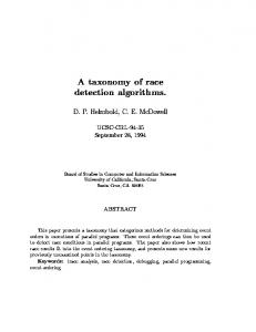
Concerning rule (3), let’s first notice that this rule only concerns inequalities of the form x ≤ y, that it, zero-weighted arcs in the potential graph. Thus, the propagation of rule (3) can be done on a restriction of the potential graph to zeroweighted arcs, and where nodes corresponding to equal variables are merged: let us note G• = (V • , A• , E • ) this reduced graph, where (V • , A• ) is the directed acyclic graph of zero-weighted arcs, and (V • , E • ) is the non-directed graph of disequalities. Let n• be its number of nodes. Now, taking rule (3) into account boils down to propagating an irreflexive and symmetric relation along an order relation. This propagation can be written on G• as follows:  (v1 , v2 ) ∈ A• , (v2 , v3 ) ∈ A• =⇒ (v1 , v3 ) ∈ E • (v1 , v2 ) ∈ E • ∨ (v2 , v3 ) ∈ E • and is a kind of transitive closure. Among the numerous algorithms for transitive closure, Koubeck’s algorithm [GK79] is particularly interesting, since its worstcase complexity is O((n• )2 n•r ) (where n•r is the number of arcs of the transitive reduction of the graph) and its average complexity is O((n• )2 log n• ) [Sim88]. A more recent paper evaluate it to O((n• )2 ) [SCC93]. Figure 6(a) shows an example of mixed graph, and Figure 7 gives our version of Koubeck’s algorithm, adapted to solve our closure problem. The only change is that the result Φ(v) of the algorithm is no longer the set of nodes reachable from v, but its partitioning into 2 sets: the set Φ1 (v) of nodes which are reachable from v by some path traversing an arc doubled by a disequality edge, and the set Φ2 (v) of other reachable nodes. The application of the algorithm is illustrated in

1

2

0

4 3 6

(a)

5

v ∈V• Φ(v) = Φ1 (v), Φ2 (v) 6 (∅ , {6}) 5 (∅ , {5}) 4 ({5} , {4}) 3 ({5, 6} , {3, 4}) 2 ({5, 6} , {2, 3, 4}) 1 ({2, 3, 4, 5, 6} , {1}) 0 ({2, 3, 4, 5, 6} , {0, 1}) (b)

Figure6. (a) A mixed graph G• = (V • , A• , E • ), labelled in topological order, and (b) the edges to propagate with respect to the order described by arcs, for each node v in Φ1 (v)

Figure 6(b). Notice the importance of considering successors of v in increasing topological order: if, when dealing with node 0, we start with node 3 instead of node 1, node 3 and 4 would finally belong to both Φ1 (0) and Φ2 (0). for each v ∈ V • in decreasing topological order do Φ(v) ← (∅, {v}) ; for each successor w of v in increasing topological order do if w 6∈ Φ(v) then if (M • )6= vw then Φ1 (v) ← Φ1 (v) ∪ Φ1 (w) ∪ Φ2 (w) else Φ1 (v) ← Φ1 (v) ∪ Φ1 (w) ; Φ2 (v) ← Φ2 (v) ∪ Φ2 (w)

Figure7. Algorithm computing the propagation of disequality constraints, derived from Koubeck’s transitive closure algorithm. Worst-case complexity is O((n• )3 ) time and expected complexity is O((n• )2 log n• ) time [Sim88]

Finally, the new disequalities resulting from rule (3) are all the pairs (v, w) with w ∈ Φ1 (v) and must be symmetrically reported in the initial d DBM. Notice that these new disequalities are not subject to rule (1) and take into account rule (2). The phases of complete algorithm for computing the normal form of a d DBM are given in Figure 8. 5.2

The Arithmetic Case

Testing Emptiness. Checking constraints satisfiability in Zn is classically more difficult than in dense sets. Arithmetic satisfiability of DBMs and octagons is polynomial, but it is no longer the case when combined with disequalities. The

1 2 3 4 5 6 7 8

Apply the shortest-path closure on M ≤ (Figure 1) ; Add implicit disequality constraints (rules (1) and (2)) to M 6= (Figure 5) ; Consider G the disequal potential graph of M where the set of directed edges is restricted to those with null weight ; Compute SCC, the set of strongly connected components of the directed graph of G ; Consider G• the mixed reduced graph of G constructed on SCC ; Compute O, a topological order on the directed acyclic graph of G• ; Apply the disequality propagation algorithm (rule (3)) on G• with respect to O (Figure 7) ; Add induced disequality constraints into M 6=

Figure8. Abstract algorithm of the closure of a d DBM M in the dense case. Runs in O(n3 ) time

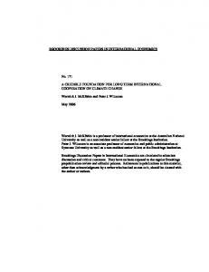
d DBM of Figure 3 illustrates the problem: it has solutions in R3 or Q3 , but not in Z3 , since we can’t find three distinct integers between 1 and 2. The complexity of the emptiness problem in arithmetic was studied by [RI80], who showed its NP-completeness by a reduction of the 3-coloration of graphs problem. A brute force technique consists in considering separately, for each disequality x − y 6= 0, the cases x − y ≤ −1 and x − y ≥ 1. This leads, for d disequalities, to 2d problems of emptiness for classical DBMs. [SW02] suggests an improvement, allowing to decrease the number d of considered disequalities: they define an “inert” disequality, as a disequality which either eliminates alone all solutions of the system of inequalities or cannot participate in the absence of such solutions. Lassez theorem states that, in the dense case, all disequalities are inert. For our restricted disequalities, some inert disequalities can be easily detected in the arithmetic case: if some variable vi involved in a disequality is not bounded by the system of inequalities (which can ≤ ≤ be checked in constant time, by checking if either M i0 or M 0i is +∞), then the disequality is inert: either it contradicts an equation, or it can be discarded in the emptiness check. Normal Form. The key novelty, in the arithmetic case, is that disequalities may involve a narrowing of the bounds in inequalities: (x − y ≤ 0 ∧ x 6= y) ⇒ (x − y ≤ −1). Since narrowed inequalities may in turn involve new narrowings, making explicit all the consequences of a d DBM is clearly an iterative process. Figure 9 shows an example of such an iterative computation: each rewriting consists of a narrowing followed by an update of weights by Floyd-Warshall; the first rewriting corresponds to the narrowing (y −x ≤ 0 ∧ x 6= y) ⇒ (y −x ≤ −1), which involves an update of z − x ≤ 1 into z − x ≤ 0 ; this new inequality is narrowed in turn into z − x ≤ −1, which involves an update of y − x ≤ −1 into y − x ≤ −2 (2nd rewriting). A brute force algorithm, shown in Figure 10 performs the computation in O(n5 ). In this algorithm, Dense-Closure stands for the computation of the normal form in the dense case, or, more efficiently, only steps 1 (Floyd-Warshall on inequality

x

z 1 −1

x

z 0 −1

1

x

y

−1 −1

1

−1

0

z 1

−2 y

y

Figure9. Propagation of disequality constraints in the arithmetic case

matrix) and 2 (propagation of rules (1) and (2)) of the algorithm of Figure 8. As a matter of fact, in the arithmetic case, rule (3) is taken into account by iterative applications of narrowing of inequalities and application of Floyd-Warshall.

repeat M ← Dense-Closure(M ) ; ≤ 6= to narrow ← {(i, j) | Mij = 0 ∧ Mij }; forall (i, j) ∈ to narrow do ≤ Mij ← −1 until to narrow = ∅ ; Figure10. Closure algorithm of d DBM M in arithmetic case

Nevertheless, this algorithm can be improved by performing weight changes from 0 to −1 on the fly, during the application of Floyd-Warshall. Remark. The opposite potential graph is the closure of the one of Fig. 3(c). Although it does not contain any negative cycle, it represents an empty domain in arithmetic. It shows that testing the emptiness of the domain described by a d DBM defined in Z is harder than computing its normal form.

6 6.1

1

x

−1 1

y

1 2

2

0 −1

−1 1

1

2 1

z

Operators on d DBMs The Lattice of d DBMs

We note M the set of d DBMs, with a least element ⊥ added (representing the empty set, D(⊥) = ∅). M is partially ordered as follows: M v M0 ⇔



either M = ⊥ or M, M 0 6= ⊥, M E M 0

The greatest d DBM, denoted > is such that, ∀i, j = 0 . . . n − 1, >≤ ij = if i = 6= j then 0 else + ∞, and >ij = false. Lattice Operators. Let M, M 0 be two d DBMs in normal form. Let us note: " ˇ = M

ˇ ≤ = max(M ≤ , M 0 ≤ ) M ij ij ij ˇ 6= = M 6= ∨ M 0 6= M ij ij ij

"

# ,

ˆ = M

ˆ ≤ = min(M ≤ , M 0 ≤ ) M ij ij ij ˆ 6= = M 6= ∧ M 0 6= M ij ij ij

#

Then the least upper bound M t M 0 and the greatest lower bound M u M 0 are defined by:    M if M 0 = ⊥ ˆ )=∅ ⊥ if M = ⊥ or M 0 = ⊥ or D(M 0 M t M = M 0 if M = ⊥ , M u M 0 = ˆ otherwise  ˇ M M otherwise 6.2

Other Operators

Existential quantification and projection. Both operations consist in losing all information, in a d DBM M , about a variable x, while keeping the remaining information about other variables. In the quantification ∃x, M , the variable x is eliminated, while in the projection M ↓x , x is left as a non-constrained variable. Both operations need first a normalization of M , to gather all the consequences ≤ 6= on other variables, then ∃x, M is obtained by suppressing in M and M all the rows and columns corresponding to x, while for M ↓x , the rows and columns ≤ 6= corresponding to x in M (resp., in M ) must be filled with ’+∞’ (resp., with ’false’). Post-condition of an assignment. As usual, the abstract post-condition of an assignment x ← e can be computed using existential quantification (z is a fresh variable) and projection: [x ← e](M ) = ∃z ((M ∧ (z = e)) ↓x ∧ (x = z)) It will be precise when the expression e is of the form y + c or c; otherwise, the term (z = e) cannot be expressed in a d DBM, and all information about x is lost, unless some ad-hoc treatment is applied: for instance, if M includes the constraints (x = y), (z 6= 0) then the precision of [x ← x + z](M ) can be improved with (y 6= x). Conditions. In order to propagate d DBMs over conditional statements, we must define the abstraction of conditions. Obviously, only conditions expressible in d DBMs can be precisely taken into account, i.e., conjunctions of conditions of the form x − y ≤ c, ±x ≤ c, x 6= y, x 6= 0. The lattice operator t can be used to approximate disjunctions of such conditions. Ad-hoc interpretations can be defined for some other kinds of conditions, but otherwise the abstraction will be >.

Widening operator. The lattice of classical DBMs being of infinite depth, so is the lattice of d DBMs; so we must define a widening operator. However, there is no infinite chain of disequality matrices. Consider M, M 0 ∈ M, with M v M 0 and M 0 in normal form (this always improves the precision of the operator). The widening M ∇M 0 will remove, as usual, the inequalities of M which are not satisfied in M 0 , but all the disequalities in M 0 can be kept in the result. In fact, our exact definition depends of V: of course, we want to specialize the bounds 0 and −1 in the arithmetic case in order to preserve the constraint (x ≤ y) when we widen (x < y) by this constraint. When V = Z, without this specialization, the inequality (x − y ≤ 0) would get lost in (x − y ≤ −1, x − y 6= 0) ∇ (x − y ≤ 0). As usual, M ∇M 0 is M 0 , if M = ⊥. Otherwise, M ∇M 0 = (M ∇≤ , M 06= ), where ∀i, j = 0 . . . n−1,  ≤ ≤ ≤   Mij if M 0 ij ≤ Mij ∇≤ ≤ ≤ Mij = M 0 ij if Mij = −1, M 0 ≤ ij = 0 and V = Z   +∞ otherwise

7

Application to Program Analysis

A prototype analyzer has been implemented, using the general fixpoint computation engine developed by Bertrand Jeannet for NBAC [Jea]. Figure 11 gives the results of the analysis of a very simple, ad-hoc program. The goal was to show that (x 6= y) at point (3).

read(x) ; read(y) ; if (x = y) then (2) OK else while true do (3) if (x = y) then ERR ; read(z) ; (4) if (x y ERR ⊥ (1)

Figure11. Example of a toy program and the obtained results

Other simple programs have been successfully analyzed, e.g.: a circular buffer, where we show that, when the buffer is neither full nor empty, the indexes of the first and last elements are always different; the bakery algorithm, which is proved, by means of invariants of the form pi 6= 0, to properly synchronize two processes p1 and p2 .

Beyond these simple examples, our abstract domain of d DBMs can be used in other kinds of analyzes: for instance, in Deutsch’s pointer analysis [Deu94], d DBMs could be used instead of other classical abstract domains, to represent the possible aliases between two linked lists.

8

Conclusion

We have proposed a new numerical domain dealing with both potential constraints and disequalities between variables. The complexity is O(n3 ) when variables take their values in a dense set. In the arithmetic case, apart from the emptiness problem which is well-known to be exponential, other operations are in O(n5 ). Our very rough prototype did not allow large examples to be dealt with, so our next task will be to integrate the new domain in an existing analyzer, in particular to check its effectiveness for alias analysis. Another short-term perspective is to extend this work to octagons [Min01], where disequalities of the form (x 6= −y) could also be expressed. Moreover, in this paper, we wanted, as far as possible, not to increase the complexity of the DBM domain, but of course, if this constraint is released, we could consider more general disequalities.

References [ACD93]

R. Alur, C. Courcoubetis, and D.L. Dill. Model-checking in dense real-time. Information and Computation, 104(1):2–34, 1993. [Bou93] F. Bourdoncle. Abstract debugging of higher-order imperative languages. In PLDI’93, pages 46–55, New York, 1993. [CC76] P. Cousot and R. Cousot. Static determination of dynamic properties of programs. In 2nd Int. Symp. on Programming, pages 106–130. Dunod, Paris, 1976. [CC04] R. C. Claris´ o and J. Cortadella. Verification of parametric timed circuits using octahedra. In Designing correct circuits, DCC’04, Barcelona, 2004. [CH78] P. Cousot and N. Halbwachs. Automatic discovery of linear restraints among variables of a program. In POPL’78, pages 84–96, jan 1978. [CLRS90] T. H. Cormen, C. E. Leiserson, R. L. Rivest, and C. Stein. Introduction to Algorithms. The MIT Press, Cambridge, Massachusetts, 1990. [Deu94] A. Deutsch. Interprocedural may-alias analysis for pointers: beyond klimiting. In PLDI’94, pages 230–241, 1994. [Dil89] D. L. Dill. Timing assumptions and verification of finite-state concurrent systems. In Automatic Verification Methods for Finite State Systems, pages 197–212. LNCS 407, Springer-Verlag, 1989. [GK79] A. Goralcikov´ a and V. Koubek. A reduct-and-closure algorithm for graphs. In MFCS, pages 301–307, 1979. [Gra91] P. Granger. Static analysis of linear congruence equalities among variables of a program. In CAAP ’91, pages 169–192, 1991.

[HS97]

W. Harvey and P. J. Stuckey. A unit two variable per inequality integer constraint solver for constraint logic programming. In Twentieth Australasian Computer Science Conference, ACSC’97, pages 102–111, February 1997. [HS03] W. Harvey and P. J. Stuckey. Improving linear constraint propagation by changing constraint representation. Constraints, 8(2):173–207, 2003. [Imb93] J.-L. Imbert. Variable elimination for generalized linear constraints. In ICLP, pages 499–516, 1993. [Jea] B. Jeannet. The NBAC verification/slicing tool. http://www.inrialpes.fr/pop-art/people/bjeannet/nbac/. [JHR99] B. Jeannet, N. Halbwachs, and P. Raymond. Dynamic partitioning in analyses of numerical properties. In SAS’99, Venezia, September 1999. [Kar76] M. Karr. Affine relationships among variables of a program. Acta Informatica, 6:133–151, 1976. [LM92] J.-L. Lassez and K. McAloon. A canonical form for generalized linear constraints. J. Symb. Comput., 13(1):1–24, 1992. [LPWY99] K. G. Larsen, J. Pearson, C. Weise, and Wang Yi. Clock difference diagrams. Nordic J. of Computing, 6(3):271–298, 1999. [Mas93] F. Masdupuy. Semantic analysis of interval congruences. In International Conference on Formal Methods in Programming and Their Applications, pages 142–155, 1993. [Min01] A. Min´e. The octagon abstract domain. In AST 2001 in WCRE 2001, IEEE, pages 310–319. IEEE CS Press, October 2001. [Min02] A. Min´e. A few graph-based relational numerical abstract domains. In SAS ’02: Proceedings of the 9th International Symposium on Static Analysis, pages 117–132, London, UK, 2002. Springer-Verlag. [MLAH99] J. B. Møller, J. Lichtenberg, H. R. Andersen, and H. Hulgaard. Difference decision diagrams. In CSL ’99, pages 111–125. Springer-Verlag, 1999. [MR05] L. Mauborgne and X. Rival. Trace partitioning in abstract interpretation based static analyzers. In ESOP 2005, Edinburgh, April 2005. [Pug98] J.-F. Puget. A fast algorithm for the bound consistency of alldiff constraints. In AAAI ’98/IAAI ’98: Proceedings of the fifteenth national/tenth conference on Artificial intelligence/Innovative applications of artificial intelligence, pages 359–366, Menlo Park, CA, USA, 1998. American Association for Artificial Intelligence. [PW98] W. Pugh and D. Wonnacott. Constraint-based array dependence analysis. ACM Trans. Program. Lang. Syst., 20(3):635–678, 1998. [RI80] D. J. Rosenkrantz and H. B. Hunt III. Processing conjunctive predicates and queries. In VLDB, pages 64–72, 1980. [SCC93] K. Simon, D. Crippa, and F. Collenberg. On the distribution of the transitive closure in a random acyclic digraph. In ESA ’93, pages 345–356. Springer-Verlag, 1993. [Sim88] K. Simon. An improved algorithm for transitive closure on acyclic digraphs. Theor. Comput. Sci., 58(1-3):325–346, 1988. [SISG06] S. Sankaranarayanan, F. Ivanˇci´c, I. Shlyakhter, and A. Gupta. Static analysis in disjunctive numerical domains. In SAS’06, Seoul, Korea, August 2006. [SW02] Robert Seater and David Wonnacott. Efficient Manipulation of Disequalities During Dependence Analysis. In LCPC ’02: Proceedings of the 15th international workshop on Languages and Compilers for Parallel Computing, volume 2481, pages 295–308, December 2002.