An Abstract Dual Propositional Model Counter Armin Biere1
Steffen H¨olldobler2,3
∗
Sibylle M¨ohle2
1
Johannes Kepler University Linz, Austria Technische Universit¨at Dresden, Dresden, Germany North-Caucasus Federal University, Stavropol, Russian Federation 2
3
[email protected]
[email protected]
[email protected]
Abstract Various real-world problems can be formulated as the task of counting the models of a propositional formula. This problem, also called #SAT, is therefore of practical relevance. We present a formal framework describing a novel approach based on considering the formula in question together with its negation. This method enables us to close search branches earlier. We formalize a non-dual variant and argue that our framework is sound.
1
Introduction
The problem #SAT consists in determining the number of models of a propositional formula. Applications can be found in a variety of real-world domains, such as reasoning [Rot96, LvBP06], model-based diagnosis of physical systems [Kum02], product configuration in the automotive industry [KZK10], planning [PBDG05], and frequent itemset mining [HLM12]. The breadth of these applications emphasizes the practical relevance of #SAT. Birnbaum and Lozinskii presented an algorithm for counting propositional models based on the Davis Putnam Procedure [BL99]. In [JP00], the authors extend this method by splitting the formula in question into subformulae over disjoint sets of variables. The model count is then obtained by multiplying the model counts of these subformulae. In Cachet [SBB+ 04] clause learning and component caching are combined. sharpSAT [Thu06] builds upon Cachet introducing a new component caching scheme. Projected model counting was implemented in [KMM13, ACMS15]. Finally, in [BSB15], a parallel approach is implemented. With a similar motivation as [FSB16] but for #SAT instead of QBF in the spirit of [NOT06], we present a formal framework describing a #SAT solving procedure based on DPLL, called Abstract Dual #DPLL, and a formalization of a non-dual variant and argue that our framework is sound. The basic idea of our dual approach consists in executing DPLL on a formula as well as on its negation. In our counting algorithm, we follow the main idea presented in [BL99]. We implement our framework in SWI-Prolog [WSTL12] making use of the PIE system [Wer16]. First experiments showed the suitability of our approach. While a dual approach was addressed in QBF [GSB13, FSB16], we are not aware of any work on #SAT aiming in this direction. The paper is structured as follows: After giving some background information, in Sect. 3 we present the rules for dual propositional model counting underlying our counting procedure. In Sect. 4 we introduce our framework and argue about its soundness. By means of an example, in Sect. 5 we demonstrate the operation of our framework as well as of a non-dual variant, before in Sect. 6 we conclude and point out future work. Our notation is based on the one introduced in [HMPS14]. ∗ The authors are listed in alphabetical order. cc 2017 Copyright the paper’s authors. Copying permitted for private and academic purposes. Copyright
by thebypaper’s authors. Copying permitted for private and academic purposes. In: S.A.H¨ o lldobler,B.A.Coeditor Malikov, (eds.): C. Wernhard (eds.): of YSIP2 – Proceedings of the Second Country, Young Scientist’s International Workshop Editor, Proceedings the XYZ Workshop, Location, DD-MMM-YYYY, published at on Trends in Information Processing, Dombai, Russian Federation, May 16–20, 2017, published at http://ceur-ws.org. http://ceur-ws.org
1 17
2 2.1
Preliminaries Propositional Satisfiability and Model Counting
Let V be a fixed finite set of propositional variables. A literal L is either a variable A (positive literal ) or a negated variable ¬A (negative literal ). We denote with var(L) the variable of L. The complement L of a literal L is its negation, i.e., L = ¬A if L = A, and L = A if L = ¬A. A propositional formula F over variables in V is in conjunctive normal form (CNF), if it is a conjunction of clauses. A clause is a disjunction of literals. We denote with VF the set of variables occurring in F . We define an interpretation I as a mapping from the set of variables V to the set of truth values {>, ⊥}. If I(A) ∈ {>, ⊥} for all A ∈ V, then I is called a total interpretation. Otherwise, I is said to be a partial interpretation. An interpretation may be represented by a sequence of literals containing no pair of complementary literals where each literal occurs at most once. An empty sequence is represented by (). Let I = (L1 , . . . , Lm ) be a sequence of literals representing an interpretation over V. We say that a literal L ∈ I iff L = Lk for a k ∈ {1, . . . , m}. Let I 0 = (Lm+1 , . . . , Ln ) be another sequence of literals representing an interpretation over V. We define the concatenation of I and I 0 as II 0 = (L1 , . . . , Ln ). With ILI 0 = (L1 , . . . , Lm , L, Lm+1 , . . . , Ln ) we denote the concatenation of I, L, and I 0 . Note that for II 0 and ILI 0 to represent interpretations, they have to meet the requirements given above. We interpret a sequence of literals over different variables also as a set of literals as well as the (possibly partial) interpretation which sets all its literals to true and vice versa. In the rest of this paper, I will denote an interpretation assuming an appropriate representation. An interpretation I satisfies a positive literal L with variable A, in symbols I |= L, iff I(A) = >. Analogously, I satisfies a negative literal L with variable A iff I(A) = ⊥. Since a clause C is a disjunction of literals, I |= C iff I |= L for a literal L ∈ C. Analogously, I |= F iff I |= C for all clauses C of a formula F , since F is defined as a conjunction of clauses. Whenever I |= F , we say that I is a model for F where I can be partial representing a partial model or total representing a total model. The model count #F of a formula F corresponds to the number of total models of F . Two formulae F and G are semantically equivalent, denoted by F ≡ G, iff for all interpretations I the following holds: I |= F iff I |= G. Thus, two formulae are semantically equivalent iff they have the same models. The reduct of a formula F with respect to an interpretation I is given by F |I = {C|I | C ∈ F and C ∩ I = ∅}, / I}. Let F = (x1 )∧(x2 ∨x3 ) be a formula over V = {x1 , x2 , x3 }. In set notation, where C|I = {L | L ∈ C and L ∈ F = {{x1 }, {x2 , x3 }}. Let I = {x1 , ¬x2 } be an interpretation over V. Then, F |I = {{x3 }}. Whenever F |I = ∅, I is a model of F . We say that I satisfies F and may refer to I as a satisfying interpretation where adequate. If ∅ ∈ F |I , we say that a conflict arises in F |I or that I falsifies F and call I a falsifying interpretation. In our example, I neither satisfies nor falsifies F . 2.2
The Davis Putnam Logemann Loveland Procedure
The Davis Putnam Logemann Loveland (DPLL) procedure [DLL62] is based on the Davis Putnam Procedure (DPP) [DP60] and conducts a systematic search in the space of all possible interpretations. This space can be visualized as a binary search tree where each node represents a partial interpretation and each leaf represents a total interpretation. DPLL can be visualized as a depth-first tree search based mainly on unit propagation, decisions, and backtracking. Let F be a formula and I an interpretation over V. If during search a unit clause {L} occurs in F |I , the unit literal L must be assigned the value > to make I satisfy F . This is ensured by unit propagation. L is called propagation literal, and we say that L’s value is implied by F |I . If there is no unit clause in F |I , a decision literal L is chosen and assigned a value. If I falsifies F , backtracking occurs, i.e., all assignments up to the latest decision are undone and the value of the decision literal flipped. The search continues with I modified accordingly. For a more detailed description we refer to [DP09]. 2.3
Counting Models by Means of the Davis Putnam Procedure
Let F be a formula and I an interpretation over variables V. By means of a decision with respect to a literal L, the set of models of F is split into two disjoint sets. In one I(L) = >, in the other I(L) = ⊥. Hence, #F |I = #F |I∪{L} + #F |I∪{L} . Based on this observation, a method for counting models based on the Davis Putnam procedure [DP60] was presented in [BL99]. The corresponding pseudocode is depicted in Algorithm 1. It is important to note that, unlike in SAT solving, after determining a satisfying interpretation, the search continues until the entire search space has been processed. The model count is built recursively according to the
2 18
function CDP(F , |V|) . F formula over a set of variables V if F is empty then . F is satisfiable return 2|V| else if F contains an empty clause then . F is unsatisfiable return 0 else if F contains a unit clause {L} then . Unit propagation return CDP(F |{L} , |V| − 1) else choose a variable A ∈ V return CDP(F |{A} , |V| − 1) + CDP(F |{¬A} , |V| − 1) end if end function Algorithm 1: Counting by Davis-Putnam (CDP) [BL99]. Dec:
P I M ;Dec P I L˙ M
var(L) ∈ V
iff
0
NB>:
˙ 0 M ;NB> P IL M + 2|V|−|ILI | P I LI iff 0 0 P |ILI = ∅ and I contains only propagation literals
NB⊥:
˙ 0 M ;NB⊥ P IL M P I LI ∅ ∈ P|
End>:
ILI 0
End⊥:
iff
0
and I contains only propagation literals
P I M ;End> M + 2|V|−|I|
P |I = ∅
and {L, L} ∩ I = ∅
iff
and I contains only propagation literals
P I M ;End⊥ M
iff
∅ ∈ P |I
and I contains only propagation literals
Figure 1: Rules in Abstract #DPLL. P is a CNF formula over variables V, I and I 0 are interpretations over disjoint sets of variables, L is a literal and M ∈ N. The procedure is based on DPLL combined with naive backtracking and terminates when the entire search space has been processed. computation discussed in the previous paragraph. We now present rules to determine #F based on Algorithm 1. Let P be a CNF formula over V such that P ≡ F . #F |I = #P |I = 2m with m = |V| − |I| representing the number of unassigned variables. Now #P |I can be computed by the following rules: Whenever I falsifies P , #P |I = 0; whenever I satisfies P , #P |I = 2|V|−|I| ; whenever #P |I is undefined, then #P |I = #P |I∪{L} + #P |I∪{L} , where var(L) ∈ V and {L, L} ∩ I = ∅. 2.4
An Abstract Framework for Propositional Model Counting
Let F be a formula over V and P be a CNF formula over V such that P ≡ F . We describe Abstract #DPLL as a state transition system (S, ;) with a set of states S and a binary transition relation ; ⊆ S×S. The set of states is defined by S := N ∪ {P I M | P is a CNF formula such that P ≡ F , I is an interpretation, and M ∈ N}, and ; := {;Dec , ;NB> , ;NB⊥ , ;End> , ;End⊥ }. In this context, P is called working formula, I is called working interpretation, and M is called working number of models. The initial state is defined by P () 0. The terminal state is #P = #F . L˙ denotes a decision literal, i.e., a literal which was assigned a value by a decision. Analogously, L denotes a propagation literal. The rules are presented in Fig. 1. By means of the Dec rule, the working interpretation is extended by an unassigned decision literal L˙ whose variable occurs in V. Naive backtracking is applied whenever the working interpretation either satisfies or falsifies P and if it contains a decision literal, i.e., not not all possible interpretations have been tested yet. In the former case, the model count has to be incremented by 2m , where m represents the number of unassigned variables (NB>). In the latter case, the model count remains unchanged (NB⊥). The procedure terminates when I either satisfies (End>) or falsifies (End⊥) P and does not contain any decision literal, i.e., all possible interpretations
3 19
have been tested. The model count is updated accordingly. If our framework is sound, every implementation which can be modeled by means of it is sound as well. This comprises optimizations, such as unit propagation. Restricting our framework to a minimal set of rules simplifies the presentation since less cases have to be distinguished and reasoned about.
3
Counting Models by Taking into Account the Negated Formula
Let F be a formula over variables V, P and N be CNF formulae over V such that P ≡ F and N ≡ ¬F , respectively. Then, #F = #P = 2|V| − #N . Further let I be an interpretation over V. For the reduct F |I the same observation holds: #F |I = #P |I = 2|V|−|I| − #N |I , where |V| − |I| represents the number of unassigned variables. Given F , P , N , and V, we define the counting algorithm c taking as input I: R1: R2: R3: R4: R5:
c(I) = 0 c(I) = 2|V|−|I| c(I) = 2|V|−|I| c(I) = 0 c(I) = c(I ∪ {L}) + c(I ∪ {L}) where var(L) ∈ V and {L, L} ∩ I = ∅
if if if if else
∅ ∈ P |I P |I = ∅ ∅ ∈ N |I N |I = ∅
Conflict in P |I I |= P Conflict in N |I I |= N
If a conflict in P |I arises, I can not be extended to any total model for F , and the model count is 0 (R1). Whenever I |= P , I can be extended to 2|V|−|I| total models for F , where |V| − |I| is the number of unassigned variables (R2). In case of a conflict in N |I , I is a model for F and can be extended to 2|V|−|I| total models for F (R3). Whenever I |= N , I can not be extended to a total model for F , and the model count is 0 (R4). If both P |I and N |I are undefined, #F |I = #P |I∪{L} + #P |I∪{L} (R5) [BL99]. Unit propagation in P |I can be simulated by rules R5 and R1: c(I) = c(I ∪ {L}) + c(I ∪ {L}) = c(I ∪ {L}) | {z }
if
{L} ∈ P |I
(1)
0
{L} is a unit clause in P |I , and therefore L must be set to > for I ∪ {L} to satisfy P . This implies that I ∪ {L} falsifies P , i.e., c(I ∪ {L}) = 0 according to rule R1. Unit propagation in N |I can be simulated by rules R5 and R3: c(I) = c(I ∪ {L}) + c(I ∪ {L}) = c(I ∪ {L}) + 2|V|−|I∪{L}| | {z }
if
{L} ∈ N |I
(2)
2|V|−|I∪{L}|
{L} is a unit clause in N |I , and therefore L must be set to > for I ∪ {L} to satisfy N . This implies that I ∪ {L} falsifies N , i.e., I ∪ {L} satisfies F and can be extended to 2|V|−|I∪{L}| total models for F according to rule R3.
4
Abstract Dual #DPLL
Let F be a formula over variables V, P and N be CNF formulae over V such that P ≡ F and N ≡ ¬F , respectively. Note that in particular VF = VP = VN = V. Let I be an interpretation. Clearly, I |= P iff I 6|= N and vice versa. P and N are passed to a DPLL [DLL62] solver which works on both formulae simultaneously. The model count is computed according to the rules introduced in Sect. 3. If a conflict in P |I arises, I can not be extended to a total model for F , and the model count is 0. Whenever P |I = ∅, I satisfies P and can be extended to 2m total models for F , where m is the number of unassigned variables. This model count is added up to the number of models found so far. In both cases, the solver backtracks chronologically and flips the value of the decision literal turning it into a propagation literal. The search terminates if I contains no decision literal, indicating that the whole search space has been processed. If a conflict arises in N |I , I is a model for F and can be extended to 2m total models for F , where m is the number of unassigned variables. This model count is added up to the number of models found so far. Whenever N |I = ∅, I satisfies N and can not satisfy F . In both cases, the solver backtracks chronologically and flips the value of the decision literal turning it into a propagation literal. The search terminates if I does not contain any decision literal, indicating that the whole search space has been processed.
4 20
Dec: NB>:
P N I M ;Dec P N I L˙ M
˙ 0 M ;NB> P N IL M + 2|V|−|ILI 0 | P N I LI (∅ ∈ N |
ILI 0
NB⊥:
var(L) ∈ V
iff
or P |
ILI 0
= ∅)
(∅ ∈ P |
or N |
ILI 0
= ∅)
iff
0
and I contains only propagation literals
˙ 0 M ;NB⊥ P N IL M P N I LI ILI 0
and {L, L} ∩ I = ∅
iff
0
and I contains only propagation literals
End>:
P N I M ;End> M + 2|V|−|I| iff (∅ ∈ N |I or P |I = ∅) and I contains only propagation literals
End⊥:
P N I M ;End⊥ M
(∅ ∈ P |I or N |I = ∅)
iff
and I contains only propagation literals
Figure 2: Rules in Abstract Dual #DPLL. P and N are CNF formulae over V such that N ≡ ¬P , I and I 0 are interpretations over disjoint sets of variables, L is a literal, and M ∈ N. The procedure is based on DPLL combined with naive backtracking and terminates as soon as the entire search space has been processed. Whenever both P |I and N |I are undefined, an unassigned literal L is chosen and assigned a value becoming a decision literal. The search continues with I extended by L. In our version of DPLL, every node is visited at most once, and there is no need to remember the models found so far, e.g., by adding blocking clauses (i.e., the negated models) to P to avoid finding models several times. This ensures that the model count returned by the algorithm corresponds to the number of models of F . 4.1
States and Transition Relations
Based on Abstract #DPLL introduced in Sect. 2.4, we describe Abstract Dual #DPLL as a state transition system (S, ;) with set of states S and transition relation ; ⊆ S ×S as follows: S := N ∪ {P N I M | P , N are CNF formulae with P ≡ F and N ≡ ¬F , I is an interpretation, M ∈ N}
; := {;Dec , ;NB> , ;NB⊥ , ;End> , ;End⊥ }
In this context, P and N are called working formulae, I is called working interpretation, and M is called working model count. The initial state is defined by P N () 0. The terminal state is the model count of P and therefore of F . We denote with L˙ a decision literal, i.e., a literal which was assigned a value by a decision. Analogously, L denotes a propagation literal. The rules are presented in Fig. 2. 4.2 Dec
Rules I is extended by an unassigned decision literal L˙ whose variable occurs in V.
NB> Naive backtracking is applied whenever the working interpretation either satisfies P or falsifies N and ˙ In this case, the working interpretation has the form I LI ˙ 0 . The model count is contains a decision literal L. |V|−|ILI 0 | , according to rules R2 and R3 specified in Sect. 3. incremented by 2 NB⊥ Naive backtracking is applied whenever the working interpretation either satisfies N or falsifies P and ˙ In this case, the working interpretation is of the form I LI ˙ 0 . The model count contains a decision literal L. remains unaffected, see rules R1 and R4 specified in Sect. 3. End> The procedure terminates with a satisfying interpretation I. This is the case when I either satisfies P or falsifies N and contains no decision literal. The model count is incremented by 2|V|−|I| , according to rules R2 and R3 specified in Sect. 3. End⊥ The procedure terminates with a falsifying interpretation I. This is the case when I either satisfies N or falsifies P and contains no decision literal. The model count remains unaffected, according to rules R1 and R4 specified in Sect. 3.
5 21
4.3
Unit Propagation
Unit propagation is simulated by the Dec and NB> or NB⊥ rule, respectively, according to Sect. 3. In particular, the Dec rule may be applied if a unit clause {L} occurs in either P |I or N |I . Unit Propagation in P |I Let’s assume that after setting L to >, during the further execution of the procedure a conflict or empty reduct results in either P |I or N |I . Naive backtracking is performed, M is updated, and L’s value is flipped according to rules NB> or NB⊥ (see Sect. 4.2). Since L is a unit literal in P |I , the unit clause {L} in P |I becomes empty when L’s value is flipped, and IL falsifies P . Hence, #P |IL = 0. This corresponds to the second term in the sum of (1). Unit Propagation in N |I Let’s assume that after setting L to >, during executing the procedure a conflict or empty reduct results in either P |I or N |I . Naive backtracking is performed, M is updated, and L’s value is flipped according to one of the rules NB> or NB⊥ (see Sect. 4.2). Since L is a unit literal in N |I , the unit clause {L} in N |I becomes empty, and IL falsifies N . Hence, IL satisfies P , and #P |IL = 2|V|−|IL| . This corresponds to the second term in the sum of (2). 4.4
Soundness
To make sure that the correct model count is returned by our framework, every node in the search tree must be visited or counted exactly once. By this we mean that an ancestor u of a node v may be visited, but not v itself. This can only occur if u represents a satisfying or falsifying interpretation. In this case, all its descendants, including v, represent a satisfying or falsifying interpretation as well, and the model count determined in v includes all of them. The naive backtracking mechanism employed in our DPLL version ensures that each node in the search tree is visited at most once. Therefore, we have to show that our framework does not allow for multiple visits of nodes. The working interpretation I is extended iteratively by the Dec rule until it either satisfies or falsifies one of P or N . If I contains a decision literal, this indicates that not all combinations of truth values of the values have been tested yet. Chronological backtracking occurs and the value of the decision literal is flipped, i.e., another combination of truth values will be tested in the next step. The NB> and NB⊥ rules describe this behaviour for the case in which I is either a satisfying or falsifying interpretation, respectively. Analogously, if I contains no decision literal, all possible combinations of truth values have been tested, and the search terminates. This behaviour is addressed by the End> and End⊥ rules, where I is either a satisfying or falsifying interpretation, respectively. To prove that our framework returns the correct model count, we show that the rules presented in Sect. 4.2 update the working model count correctly. The Dec rule extends the working interpretation I by a decision literal whenever the working interpretation neither satisfies nor falsifies either P or N , thus it must not alter the number of models. In our framework, M remains unchanged when the Dec rule is applied, and the requirement holds. The NB> and End> rules are applicable, whenever the working interpretation either falsifies N or is a (possibly partial) model for P . Whenever it falsifies N , it satisfies P and can be extended to 2m models of P with m = |V| − |I| denoting the number of unassigned variables. If prior to applying one of these two rules the working model count was M , it should amount to M + 2m afterwards. The NB> and End> rules are defined accordingly. The NB⊥ and End⊥ rules are applicable, whenever the working interpretation either falsifies P or is a model for N . In both cases, it can not satisfy P and thus can not be extended to a model of P . The working model count has to remain unaffected by the application of these two rules. In our framework, this is ensured by their definition. From these arguments it follows that our framework is sound. We further implemented the framework in SWI-Prolog [WSTL12] making use of predicates defined in PIE [Wer16] for a second check of the rules. First experiments showed the suitability of our approach, while a broader evaluation is ongoing.
5
Example
We demonstrate the function of Abstract Dual #DPLL by an example. Let us consider a #SAT algorithm implementing the rules defined in Abstract Dual #DPLL introduced in Sect. 4 as well as rules UPP and UPN addressing unit propagation in P and N , respectively. Unit propagation in P can be executed if a unit clause occurs in P |I , and, according to (1), the model count is not affected. Unit propagation in N can be applied if a unit clause occurs in N |I . It modifies the model count as shown in (2). We define rules for unit propagation
6 22
using the notation of our framework to illustrate their effect. To this end, we introduce transition relations ;UPP and ;UPN , respectively. UPP: UPN:
P N I M ;UPP P N IL M
if
{L} ∈ P |I
P N I M ;UPN P N IL M + 2|V|−|IL|
if
{L} ∈ N |I
Let F be an arbitrary formula over a set of variables V, P and N be CNF formulae over V such that P ≡ F and N ≡ ¬F , respectively. Let I denote an interpretation over V and M the working model count. The empty formula is represented by ∅, the empty clause by (). In this context, I is represented by a sequence of literals. Consider as an example F = (x1 ∧ x2 ) ∨ (x3 ), where #F = 5. Then, V = {x1 , x2 , x3 }, P = (x1 ∨ x3 ) ∧ (x2 ∨ x3 ), and N = (¬x1 ∨ ¬x2 ) ∧ (¬x3 ). We assume that the variables are ordered in the following manner: x1 < x2 < x3 . For choosing the decision literal, various heuristics may be applied. The same applies to the choice of the unit literal, if several unit clauses occur. In our example we define that literals are picked in ascending order of their variable and that they are set to >. The execution trace is depicted in Table 1. Each row corresponds to an execution step with I, P |I , N |I , and M obtained by applying the rule indicated in the second column. Step 0 The system is initialized: P ≡ F , N ≡ ¬F , I = (), and M = 0. N |I contains a unit clause, namely (¬x3 ), and I neither satisfies nor falsifies either P or N . Hence, the preconditions of the UPN rule are met. Step 1 By means of the UPN rule, ¬x3 is propagated and appended to I which becomes I = (¬x3 ). M has to be increased by 2m , where m = |{x1 , x2 , x3 }| − |(¬x1 )| = 2: M = 4. I neither satisfies nor falsifies either P or N , and P |I contains two unit clauses, namely (x1 ) and (x2 ), and the preconditions of the UPP rule are met. Step 2 According to our heuristic, we choose x1 and propagate it by means of the UPP rule. I = (¬x3 , x1 ), M remains unaltered. I neither satisfies nor falsifies either P or N . Both P |I and N |I contain a unit clause each, namely (x2 ) and (¬x2 ), respectively, and the preconditions of UPP and UPN are met. Step 3 We choose to propagate (x2 ) by means of the UPP rule. I = (¬x3 , x1 , x2 ), M remains unaltered. I satisfies P and falsifies N . Since I contains no decision literals, the preconditions of both End> and End⊥ are met. Step 4 The search terminates with I = (¬x3 , x1 , x2 ) satisfying P and falsifying N with the application of the End> rule. All variables are assigned a value, M is increased by 20 = 1, and M = 5 is returned. To assess the efficiency of an algorithm based on our framework, we use the number of rules applied as performance measure without counting the initialization step. The shorter an execution trace results, the better the algorithm performs. The execution trace of our example has length 4. We now compare our dual approach with a non-dual one. To this end, let us consider a #SAT algorithm implementing the rules defined in Abstract #DPLL (see Sect. 2.4) as well as a rule UP addressing unit propagation. We introduce the transition relation ;UP . Table 1: Trace of a #SAT algorithm implementing the rules of Abstract Dual #DPLL extended by unit propagation. P and N are formulae such that N ≡ ¬P . I, P |I , N |I , and M denote the working interpretation, the working formulae and the working model count after applying the rule indicated in the second column, respectively. I is built according to the DPLL mechanism. Instead of terminating when I satisfies P , the model count is updated, naive backtracking is applied and the search continues until all decision literals are worked on. Step 0 1 2 3 4
Rule UPN UPP UPP End>
I () (¬x3 ) (¬x3 , x1 ) (¬x3 , x1 , x2 ) (¬x3 , x1 , x2 )
P |I (x1 ∨ x3 ) ∧ (x2 ∨ x3 ) (x1 ) ∧ (x2 ) (x2 ) ∅ ∅
7 23
N |I (¬x1 ∨ ¬x2 ) ∧ (¬x3 ) (¬x1 ∨ ¬x2 ) (¬x2 ) () ()
M 0 4 4 4 5
UP:
P I M ;UPP P IL M
if
{L} ∈ P |I
The execution trace of the non-dual algorithm executed on our previous example is depicted in Table 2. Step 0 The system is initialized: P ≡ F , I = (), and M = 0. I neither satisfies nor falsifies P , and the preconditions of the Dec rule are met. Step 1 The Dec rule is applied. According to our heuristics, x1 is chosen, set to > and appended to I which becomes I = (x˙1 ). The model count remains unaltered. I neither satisfies nor falsifies P , and the preconditions of the Dec rule are met. Step 2 The Dec rule is applied. According to our heuristics, x2 is chosen, I = (x˙1 , x˙2 ), and M remains unaltered. Since I satisfies P and contains two decision literals, namely (x˙1 ) and (x˙2 ), the preconditions of the NB> rule are met. Step 3 Naive backtracking is applied. The number of unassigned variables amounts to 1, and the model count is increased by 21 = 2 resulting in M = 2. The value of the decision literal x˙ 2 is flipped, i.e., x2 = ⊥, and x2 is turned into a propagation literal. I = (x˙1 , ¬x2 ) neither satisfies nor falsifies P . Since P |I contains the unit clause (x3 ), the preconditions of the UP rule are met. Step 4 Unit propagation is applied by setting x3 to >. I = (x˙1 , ¬x2 , x3 ), and P |I = ∅. I satisfies P and still contains a decision literal, namely (x1 ), hence the preconditions of the NB> rule are met. Step 5 Naive backtracking is applied. All variables were assigned a value, and the model count becomes M = 3. I = (¬x1 ) neither satisfies nor falsifies P , and P contains the unit clause (x3 ). The preconditions of the UP rule are met. Step 6 The UP rule is applied by propagating x3 . The working interpretation becomes I = (¬x1 , x3 ). It satisfies P and contains no decision literal meeting the preconditions of the End> rule. Step 7 The execution terminates with I = (¬x1 , x3 ) satisfying P . The number of unassigned variables is 2, and M = 3 + 2 = 5 is returned. The execution trace has length 7. We show that its length depends on the decision heuristics applied. Let the order in which the decision literals are chosen be reversed. Then, in Step 1, x3 is chosen as decision literal. After backtracking in Step 2, x3 is set to ⊥ and P |I = (x1 ) ∧ (x2 ). In Step 3, x2 is propagated by means of the UP rule, and P |I = (x1 ). In Step 4, UP is applied and x2 propagated, resulting in P |I = ∅. The execution terminates in Step 5 with the application of the End> rule, and M = 5 is returned. The execution trace has length 5. Table 2: Trace of a #SAT algorithm implementing the rules of Abstract #DPLL extended by unit propagation. I, P |I and M are the working interpretation, formula and model count, respectively. During execution, I is built according to the DPLL mechanism. Instead of terminating when I satisfies P , the model count is updated, naive backtracking is applied and the search continues until all decision literals are worked on. Step 0 1 2 3 4 5 6 7
Rule Dec Dec NB> UP NB> UP End>
I () (x˙1 ) (x˙1 , x˙2 ) (x˙1 , ¬x2 ) (x˙1 , ¬x2 , x3 ) (¬x1 ) (¬x1 , x3 ) (¬x1 , x3 )
8 24
P |I (x1 ∨ x3 ) ∧ (x2 ∨ x3 ) (x2 ∨ x3 ) ∅ (x3 ) ∅ (x3 ) ∧ (x2 ∨ x3 ) ∅ ∅
M 0 0 0 2 2 3 3 5
6
Conclusion and Future Work
The problem #SAT of determining the number of models of a propositional formula has many real-world applications. In this work, we have presented a formal framework describing a #SAT solving procedure based on DPLL, called Abstract Dual #DPLL, including a formalization of a non-dual variant, called Abstract #DPLL, and argued that our framework is sound. The Abstract Dual #DPLL procedure is given by 5 simple rules which specify the decide and naive backtracking mechanisms. The application of chronological backtracking underlying naive backtracking and the framework’s compactness facilitate the investigation of the main idea, namely to consider a formula and its negation simultaneously in #SAT solving. We demonstrated the working of Abstract Dual #DPLL on an example assuming an implementation enhanced by unit propagation and compared it do a non-dual algorithm based on Abstract #DPLL enhanced by unit propagation as well. The dual algorithm performed better, i.e., less rules were executed. This is due to the fact that in Step 1 unit propagation can be executed on N |I , whereas in the non-dual version, a decision has to be taken. For every decision, at a later time point backtracking occurs. This results in a longer execution trace. In this example, the performance of the dual version does not depend from the decision heuristics applied, contrarily to the non-dual version. Today, several #SAT solvers are available. They implement various strategies, however, to our best knowledge, no dual approach has been presented yet. We implemented our framework in SWI-Prolog, and first experiments on small crafted formulae are encouraging. An interesting question is whether by Abstract Dual #DPLL stateof-the-art #SAT solvers can be modeled. relsat v2.00 [JP00] is based on DPLL, but contrarily to our framework splits the formula under consideration into subformulae over disjoint variable sets. At present, we can not model #SAT solving procedures making use of backjumping or CDCL, such as Cachet [SBB+ 04], since non-chronological backtracking and clause learning are not supported. The performance gain of some modern #SAT solvers is due to improved data structures. This aspect is not covered by our framework as we focus on algorithms. In order to model countAtom [BSB15], our framework should be extended to support parallelization. For the sake of simplicity we assume that we are given two formulae P and N over the same set of variables which are duals of each others, e.g., models of P falsify N and vice versa. This assumption is rather strong unless we allow additional variables, e.g., Tseitin variables, to encode negation [Tse68]. Let F be an arbitrary formula over variables V. We denote with T (F ) the Tseitin transformation of F . The models of T (F ) projected onto V are exactly the models of F . Therefore, our approach can be generalized to the situation in which N contains, e.g., Tseitin variables, by projecting the models of N onto the variables occurring in P . As future work, we will make our soundness arguments more precise and investigate completeness. We also plan a more extensive experimental evaluation and a detailed comparison of our dual approach with non-dual methods. We intend to extend our work to the case where the formula under consideration and its negation communicate over “inputs” by allowing, e.g., Tseitin variables. Finally, by extending our framework to model strategies implemented in state-of-the-art SAT solvers, such as conflict-driven clause learning (CDCL) [MS99], we want to combine the strengths of duality of our Abstract Dual #DPLL with the strength of modern SAT solvers to obtain a state-of-the-art model counting framework. Acknowledgements The authors acknowledge support by the Deutsche Forschungsgesellschaft (DFG) under grant HO 1294/11-1 and by the Austrian Science Fund (FWF) project W1255-N23. We also want to thank Andreas Fr¨ohlich helping us in the early brain-storming and discussing phase of this idea.
References [ACMS15] Rehan Abdul Aziz, Geoffrey Chu, Christian J. Muise, and Peter J. Stuckey. #∃SAT: Projected model counting. In SAT, volume 9340 of Lecture Notes in Computer Science, pages 121–137. Springer, 2015. [BL99]
Elazar Birnbaum and Eliezer L. Lozinskii. The good old Davis-Putnam Procedure helps counting models. J. Artif. Intell. Res. (JAIR), 10:457–477, 1999.
[BSB15]
Jan Burchard, Tobias Schubert, and Bernd Becker. Laissez-faire caching for parallel #SAT solving. In SAT, volume 9340 of Lecture Notes in Computer Science, pages 46–61. Springer, 2015.
[DLL62]
Martin Davis, George Logemann, and Donald W. Loveland. A machine program for theorem-proving. Commun. ACM, 5(7):394–397, 1962.
25 9
[DP60]
Martin Davis and Hilary Putnam. A computing procedure for quantification theory. J. ACM, 7(3):201–215, 1960.
[DP09]
Adnan Darwiche and Knot Pipatsrisawat. Complete algorithms. In Handbook of Satisfiability, volume 185 of Frontiers in Artificial Intelligence and Applications, pages 99–130. IOS Press, 2009.
[FSB16]
Katalin Fazekas, Martina Seidl, and Armin Biere. A duality-aware calculus for quantified Boolean formulas. In SYNASC, pages 181–186. IEEE Computer Society, 2016.
[GSB13]
Alexandra Goultiaeva, Martina Seidl, and Armin Biere. Bridging the gap between dual propagation and CNF-based QBF solving. In DATE, pages 811–814. EDA Consortium San Jose, CA, USA / ACM DL, 2013.
[HLM12]
Rui Henriques, Inˆes Lynce, and Vasco M. Manquinho. On when and how to use SAT to mine frequent itemsets. CoRR, abs/1207.6253, 2012.
[HMPS14] Steffen H¨ olldobler, Norbert Manthey, Tobias Philipp, and Peter Steinke. Generic CDCL - A formalization of modern propositional satisfiability solvers. In POS@SAT, volume 27 of EPiC Series in Computing, pages 89–102. EasyChair, 2014. [JP00]
Roberto J. Bayardo Jr. and Joseph Daniel Pehoushek. Counting models using connected components. In AAAI/IAAI, pages 157–162. AAAI Press / The MIT Press, 2000.
[KMM13] Vladimir Klebanov, Norbert Manthey, and Christian J. Muise. SAT-based analysis and quantification of information flow in programs. In QEST, volume 8054 of Lecture Notes in Computer Science, pages 177–192. Springer, 2013. [Kum02]
TK Kumar. A model counting characterization of diagnoses. Technical report, DTIC Document, 2002.
[KZK10]
Andreas K¨ ubler, Christoph Zengler, and Wolfgang K¨ uchlin. Model counting in product configuration. In LoCoCo, volume 29 of EPTCS, pages 44–53, 2010.
[LvBP06] Wei Li, Peter van Beek, and Pascal Poupart. Performing incremental Bayesian inference by dynamic model counting. In AAAI, pages 1173–1179. AAAI Press, 2006. [MS99]
Jo˜ ao P. Marques Silva and Karem A. Sakallah. GRASP: A search algorithm for propositional satisfiability. IEEE Trans. Computers, 48(5):506–521, 1999.
[NOT06]
Robert Nieuwenhuis, Albert Oliveras, and Cesare Tinelli. Solving SAT and SAT modulo theories: From an abstract Davis–Putnam–Logemann–Loveland procedure to DPLL(T ). J. ACM, 53(6):937– 977, 2006.
[PBDG05] H´ector Palacios, Blai Bonet, Adnan Darwiche, and Hector Geffner. Pruning conformant plans by counting models on compiled d-DNNF representations. In ICAPS, pages 141–150. AAAI, 2005. [Rot96]
Dan Roth. On the hardness of approximate reasoning. Artif. Intell., 82(1-2):273–302, 1996.
[SBB+ 04] Tian Sang, Fahiem Bacchus, Paul Beame, Henry A. Kautz, and Toniann Pitassi. Combining component caching and clause learning for effective model counting. In SAT, 2004. [Thu06]
Marc Thurley. sharpSAT - counting models with advanced component caching and implicit BCP. In SAT, volume 4121 of Lecture Notes in Computer Science, pages 424–429. Springer, 2006.
[Tse68]
G Tseitin. On the complexity ofderivation in propositional calculus. Studies in Constrained Mathematics and Mathematical Logic, 1968.
[Wer16]
Christoph Wernhard. The PIE system for proving, interpolating and eliminating. In Pascal Fontaine, Stephan Schulz, and Josef Urban, editors, 5th Workshop on Practical Aspects of Automated Reasoning (PAAR), number 1635 in CEUR Workshop Proceedings, pages 125–138, Aachen, 2016.
[WSTL12] Jan Wielemaker, Tom Schrijvers, Markus Triska, and Torbj¨orn Lager. SWI-Prolog. Theory and Practice of Logic Programming, 12(1-2):67–96, 2012.
10 26