An Access Network Architecture for Neighborhood-scale ... - CiteSeerX

An Access Network Architecture for Neighborhood-scale Multimedia Delivery Dongsu Han David Andersen † Dina Papagiannaki† Michael Kaminsky Srinivasan Seshan June 2010 CMU-CS-10-128

School of Computer Science Carnegie Mellon University Pittsburgh, PA 15213

School of Computer Science, Carnegie Mellon University, Pittsburgh, PA, USA † Intel Labs Pittsburgh, Pittsburgh, PA, USA

Keywords: access networks, video on demand, peer-to-peer, multimedia, network architecture

Abstract Internet Service Providers (ISPs) are in a constant race to meet the bandwidth demands of their subscribers. Access link upgrades, however, are expensive and take years to deploy. Many ISPs are looking for alternative solutions to reduce the need for continuous and expensive infrastructure expansion. This paper shows that there are many forms of local connectivity and storage in residential environments, and that these resources can be used to relieve some of the access network load. Making effective use of this local connectivity, however, introduces several challenges that require careful application and protocol design. We present a new system for a neighborhood-assisted video-on-demand service that reduces access link traffic by carefully placing VoD data across the neighborhood and deciding what network technology should be used to transfer it between homes. We demonstrate analytically and experimentally that this approach can reduce the access network traffic that ISPs must provision for by up to 45% while still providing high-quality service.

1

Introduction

The delivery of multimedia content is growing at a tremendous rate, increasing 76% every year on average [49]. Cisco projects that “the sum of all forms of video (TV, video on demand, Internet, and P2P) will account for over 91% of the global consumer traffic by 2013” [9]. This growth in demand has been especially hard on connectivity to the home. For example, over the last five years, Korea Telecom’s access network traffic grew by 125%, compared to 40% growth in its core [61]. These trends are driven by the desire for higher quality video, increase in the number of video titles, and changes in viewing patterns. With digital video recorders (DVRs) and on-line video services like Hulu, users now watch videos at their convenience, and “time-shifted” viewing patterns are becoming the norm [49]. Many predictions suggest that on-demand TV and video on demand (VoD) will largely replace broadcast delivery, except for specific popular live content (e.g., sports events) [21, 19]. This transition is creating painful challenges for today’s consumer ISPs whose already-strained access networks were never designed to handle this load. Unfortunately, upgrading access links is expensive and new technologies often take decades to deploy.1 As a result, access technology can vary dramatically from neighborhood to neighborhood, and even home to home. This heterogeneity means that many users lack the bandwidth they need for the latest applications—particularly VoD—while they wait for an upgrade that is still years away. There is, however, a promising way to bridge this gap. ISPs can use local storage and local connectivity to mask access bandwidth deficiencies, particularly for time-shifted VoD. ISPs already deploy and control local storage in the form of set-top boxes and DVRs. In addition, although the bandwidth between homes and the Internet is limited by the access network, there are a variety of technologies, such as 802.11 and multimedia-over-coax (MoCA), that provide high-speed connectivity between nearby homes. The combination of storage and connectivity provide an opportunity to stage content in the neighborhood during off-peak periods and share it between homes upon request. These devices and links are relatively cheap, highly capable, and much easier to deploy than new access links. However, the inter-home connectivity provided by such technologies varies across homes, and is hard to provision to meet a target level of service. It is especially painful to manage local resources and to collectively use them to provide a guaranteed service for VoD content. This paper addresses the question: given a set of local neighborhood resources, how might one build a distributed system to reduce the demands that VoD delivery places on the access network? The system must decide, based on connectivity, the bit-rate of the content, and its popularity distribution, what content to stage at each home to maximize the local sharing of content. Our system faces three challenges: First, the system must monitor and automatically adapt to local resources to use them opportunistically while supporting the bandwidth requirement of the streamed content. Second, the system must be resilient to changes in popularity and environment and adjust the placement efficiently over time. Finally, the system must be robust to failures. The system cannot, for example, rely on any given device being available, since they physically reside in users’ homes and are subject to their control. No existing systems and placement algorithms [20, 25, 52, 56] 1

For example, the twentieth century only saw four new “pipes” to the home: power lines, phone, cable, and fiber.

1

achieve all these goals simultaneously. We present the design, implementation and evaluation of a system that successfully addresses these challenges. Our system automatically adapts the content placement to the environment and maximizes local sharing of content using a placement algorithm designed for streamed content. The algorithm effectively uses varying levels of connectivity between neighbors and minimizes overhead due to popularity and environment change. We evaluate the overhead and performance of the system during the entire cycle including bootstrapping, normal operation, flash crowd, failure modes and when the system is adapting to changes. Our evaluation shows that the system can reduce the access network traffic by up to 45% and is resilient to various changes. The rest of the paper is structured as follows. Section 2 examines challenges in access network design and describes the opportunity of using local resources. In Section 3, we explore alternative designs for video delivery. We present the design of our system in Section 4, based on a novel content placement algorithm, presented in Section 5. Details on the implementation and experimental results are found in Section 6 and Section 7 respectively. Finally, we review related work in Section 9, and conclude in Section 10.

2

Motivation

In this section, we discuss the challenges of today’s access networks and the opportunities that local resources may bring.

2.1

Increasing video demand

Two trends in home video consumption increase Internet bandwidth demand: time-shifted viewing patterns and high-definition (HD) content. Time-shifted viewing of TV content through Internet video streaming sites and the use of DVRs account for a large fraction of views, and even exceed the number of broadcast TV viewers [49, 6, 10]. The advent of interactive, “connected” TV such as Google TV will accelerate the trend towards streaming. A similar transition was observed in audio from radio broadcast to MP3 players and Internet streaming [12, 10]. At the same time, HD content is gaining popularity. HD video bit-rates range from 1.5 (Web “HD”) to 40Mbps (Blu-ray) depending on the quality, while most amateur videos in YouTube and the typical setting on the Web’s most popular codec are between 300 and 500Kbps [7, 28, 53]. Our system targets high quality movies or TV content at 10Mbps which is similar to the rate of IPTV’s HD videos [7, 39]. As home displays get larger, delivering higher quality content is important because users “care less about watching YouTube videos on the big screen” than they do about watching high-quality full movies [58].

2.2

Background in Access Networks

Current networks are not designed to handle such demand. Today’s providers use designs similar to that in Figure 1, independent of their physical layer topology. The core branches to a number of

2

CO

ISP network

CO

Distribution link

Figure 1: Access network Node Node

Fiber

Headend

c o a x

Node

Tap Tap Tap

Distribution links

Figure 2: HFC network central offices (COs) that support a cluster of geographically proximal customers. In a fiber-to-thenode (FTTN) network, the distribution link is fiber and extends out to a node in the neighborhood. From this node, existing copper wire is used to connect individual homes. In a cable provider’s hybrid fiber-coaxial (HFC) network the distribution link is part fiber and part coax. Fibers extend from the headend to nodes that convert optical signal to RF signals and output the RF signal on coax cables (Figure 2). Each HFC converter node covers about 250 to 2000 homes. Coax cables from the node is split once more by taps to enter individual homes. Each tap may support 2–8 homes [2] . Aside from a pure fiber optic access network, the distribution link is a common bottleneck today because aggregation and over-subscription often happens at this layer. The National Broadband Plan (NBP) [13], for example, assumes 17:1 over-subscription at this aggregation point. However, aggressive over-subscription does not work well with streamed video; a typical DSL network designed to provide broadband Internet service to 384 subscribers can only support 27 (7%) simultaneous streams of 1Mbps video. Paradoxically, its overuse is made worse, not better, by today’s locality-aware p2p services, since often the only control point for the access network is located in the CO or headend itself: traffic between homes in the neighborhood traverses this congested distribution link twice, wasting one of the most precious resources in the quest for efficiency. In a cable provider’s HFC network, when the fiber’s capacity exceeds the demand of neighbors covered by a single node, the cable provider can split a node to provision more bandwidth to the neighborhood. As part of the node split procedure, a single node becomes two and an unlit fiber is connected to the new node. However, spare fibers that were provisioned a decade ago have run out [55]. ISPs are now forced either to install more fiber or deploy wavelength division multiplexing (WDM) units. In general, these access network upgrades are complex and expensive [55].

3

1

29.0dB, 33.0Mbps

0.9

16

13 23.0dB, 33.0Mbps

0.8

15

CDF

0.7

14

0.6

29.5dB, 33.0Mbps 18.5dB, 7.0Mbps

24.0dB, 33.0Mbps

1

29.5dB, 33.0Mbps 12 29.0dB, 33.0Mbps 12.0dB, 7.0Mbps

0.5

11

0.4 0.3

SNR > 10 dB

9

SNR > 15dB

10

SNR > 20dB 0.2 0.1 0

45.0dB, 33.0Mbps

2

3

4

5

6

7

8

9

Figure 3: SNRs

0

2

15.0dB, 7.0Mbps

41.0dB, 33.0Mbps

16.5dB, 7.0Mbps 33.5dB, 33.0Mbps 11.0dB, 7.0Mbps

3

34.5dB, 33.0Mbps 26.0dB, 33.0Mbps

29.0dB, 33.0Mbps

22.5dB, 30.0Mbps

4 7

10 11 12 13 14 15

21.0dB, 12.0Mbps

28.5dB, 33.0Mbps

SNR > 25dB 1

Number of Neighbors

2.3

22.5dB, 30.0Mbps

20.0dB, 10.0Mbps

6

15dB, 7.0Mbps 10.5dB, 7.0Mbps

5

11.5dB, 7.0Mbps

28.5dB, 33.0Mbps

17

43.0dB, 33.0Mbps

8

14.5dB, 7.0Mbps

Neighbors and Figure 4: Topology of a neighborhood mesh network

Neighborhood-Aware Networks

Although upgrades to and new deployments of access network links are rare, many other forms of connectivity, such as 802.11 and MoCA, have seen explosive growth in the neighborhood. These technologies, originally designed for connectivity within a home, can provide connectivity between homes. In this paper, we refer to the collection of resources in the neighborhood as neighborhood networks. The goal of our work is to design ISP-driven mechanisms to share the resources of a neighborhood network in order to reduce the access network bandwidth that ISPs have to provision. In this section, we describe the properties of different neighborhood networks in detail and show that ISPs could use the infrastructure that they already deploy and install for the end user to extend their network perimeter to also include the neighborhood network. Next, we explore two key elements in such an architecture: in-home devices and inter-home connectivity. Device support for storage, computation and connectivity: The notion of ISP-driven deployment is not new, and many solutions have been proposed in that context [52, 56, 20]. A key component of such deployments is the ability of the ISP to place and control storage, computation and connectivity resources. Fortunately, ISPs and cable providers often install routers, set-top boxes (STB) and DVRs for their customers as part of service agreements. For example, previous studies have shown that a significant fraction of customers have ISP-provided WiFi APs [32]. The Multimedia over Coax Alliance (MoCA), also driven by a service provider deployment model, reports that it has shipped more than 20 million units to date [2]. Cable operators are reported to have already installed DVRs in more than 30% of American homes [41]. ISPs can easily augment these devices with increased storage and communication interfaces to enhance connectivity between homes and provide space for additional content storage. Adding 1TB of storage to an existing set-top-box would cost under $80 and add a nearly negligible power draw (about 6W). Local connectivity: Our approach is to actively discover and opportunistically use connectivity between neighbors that is often under-utilized or not used at all. The effectiveness of this approach, however, relies heavily on the assumption that local connectivity can indeed provide a

4

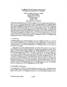
secondary high-capacity network for service providers2 . Fortunately, several options exist for highbandwidth, low-cost local communication between homes. Below, we discuss how much wireless and wired connectivity can be found between neighbors3 . Local wireless: 802.11 APs are densely deployed in residential areas [32, 16], and wireless signals often reach several neighbors. In order to assess the wireless connectivity in a neighborhood, we examined two sets of data. First, we performed a measurement study using NetStumbler in 16 different homes around Pittsburgh, Portland and Boston. Figure 3 shows the number of neighboring APs that each home can detect at different signal-to-noise ratio (SNR) thresholds. More than 85% can detect at least two APs with SNRs of 15dB or better, and over half can see five such APs. From the SNR, we can roughly infer the throughput of an 802.11g link from the results in [45]. For example, a 15dB SNR permits roughly 7 Mbps throughput, and 20dB permits 10 Mbps. Consequently, more than 75% of homes can reach two or more neighbors at 10 Mbps or faster. This type of connectivity has been used for wireless mesh networking. The second set of data we examined is from a mesh network deployment (for Internet access) by Netequality [46] using Meraki’s [43] wireless APs. Figure 4 shows the SNR measurements and estimated throughputs in this environment. Note that if the links used newer 802.11n technology, we would expect connectivity to improve significantly both in fan-out and throughput (e.g., over 100 Mbps throughput for the high signal strength links). Local wired: Recent advances in home networking use existing in-home power-line and cable TV (coax) infrastructure to provide high bandwidth connectivity for in-home devices. Wallplugged power-line communication devices deliver up to 200Mbps; Multimedia over Coax (MoCA) delivers up to 135Mbps per channel. These technologies can reach well beyond a single house (e.g., 300m for MoCA); cable and electrical wires are naturally connected when the copper from the provider splits to multiple homes [2]. Indeed, many of these technologies consider interference between homes in their design and have multiplexing mechanisms such as channel selection as well as security codes. Sometimes providers take explicit action to confine their signals to a single house, placing filters at demarcation points. Allowing interconnection between customers instead is often straightforward. The same connectivity gains apply to larger multi-dwelling units that share even more infrastructure (such as in-building Ethernet) in closer proximity. In some cases, the broadband connection itself provides the local connectivity. In a FTTN network that uses DSL technology at the last mile, the DSLAM at the node often has switching capability [11], allowing the communication between neighbors within the same DSLAM to bypass the shared distribution link.

3

VoD Delivery

Before proceeding to our solution, we describe three different architectures that are used today for video delivery: (a) broadcast TV plus DVR, (b) centralized VoD, and (c) caching at the CO 2

Otherwise, the system falls back to today’s state of the art. While there are many forms of neighborhood networks and our system design accommodates various forms of such networks, we focus on using home-networking technologies, such as 802.11 and MoCA, especially in our experimental evaluations. 3

5

(Figure 5). Positioning those architectures for VoD delivery we impose two requirements: 1) they should allow users to view any content at any time, and 2) they should reduce excessive load on the ISP’s distribution links. CO

(a) Video Server

(b)

disk disk disk homes

Video Server

(c) Video Server

CO

(d)

homes

CO cache homes disk CO disk disk homes

Local connectivity

Video Server

Figure 5: Video distribution architectures Broadcast TV plus DVR: In the broadcast TV plus DVR world, broadcast is used to deliver the same video content to all homes. Because any particular video is available only at its scheduled broadcast time, watching it at a different time requires recording and storing the content temporarily. In a VoD context, this usage model effectively translates to a prefetch mechanism where users specify what content they want to prefetch. The simple addition of a storage/DVR allows the traditional broadcast infrastructure to accommodate time-shifted viewing. The primary drawbacks of this architecture, however, are that content availability is limited by the broadcast schedule and the amount of storage on the DVR. Thus, this architecture falls short of a true VoD system, and does not satisfy sub-goal #1 (any content at any time). Centralized VoD: In the centralized VoD approach, videos are served from one central location. This location hosts servers that contain the ISP’s entire video library. Because the servers are in a centralized location, deploying and managing the system is relatively easy. The bandwidth demand on the network and video servers is high, however, because all user VoD requests go to this one location which must stream potentially different content to each user. Multicast can help minimize redundancy, but the overall demand still stresses the core network and server resources as well as the precious distribution link bandwidth. Thus, this architecture falls short of our design goal (sub-goal #2). Caching at the CO: One approach to reduce the network traffic is to place caches serving popular content closer to the homes (e.g., at the CO). This architecture reduces core bandwidth and load on the centralized video servers, but does not relieve the distribution link which is downstream from the cache. Thus, this architecture too does not satisfy sub-goal #2. Neighborhood-network: The neighborhood networking approach, shown in Figure 5(d), addresses the shortcomings of the three architectures in use today by using local resources. We propose making software changes to existing content storage devices, such as DVRs, so that they can store and share content with their neighbors using local connectivity. As a result, only the content that is not available or cannot be delivered on time from a user’s neighbors is served from the remote VoD server or a cache. In this design, ISPs proactively push content to the DVR disks using broadcast/multicast during off-peak periods for the network. This neighborhood network 6

approach has the potential to reduce the amount of bandwidth that the ISP needs to provision at its video server and at the distribution link of the access network while still providing the same level of service as traditional VoD. This architecture, however, raises several design challenges. First, the ISP must determine what content to push to any particular DVR. This data placement must take into account the local connectivity between neighbors, the popularity distribution of different content, and the possibility of failures in the local network. Second, the system has to keep the content of the DVR disks upto-date to remain effective despite the popularity change and new content introduction. Third, the system must continually monitor what inter-home connectivity options are available to inform the placement algorithm and to decide how to retrieve content from neighbors. Finally, the system must be robust to failures. The next section presents a system design that addresses these challenges.

4

Design

Based on the requirements outlined in the previous section we now describe a VoD system that uses local resources and supports a large number of videos (>10,000).

4.1

System Overview

Our proposed neighborhood VoD system has three basic (physical) components (Figure 6): centralized video servers, a centralized management server, and per-home STBs connected locally to one another and by broadband. The video servers store the master copy of all content that the system provides, and the in-home STBs have local replicas of popular content distributed across their disks. The management servers serve two functions: placement generation and directory service. Placement generation involves computing the desired placement of the content in the neighbor-nodes given system parameters such as the viewing patterns of videos and the connectivity between neighbors. The directory service maps content to a set of replicas (homes) within the neighborhood. With this set of physical resources, the logical flow of system operation is as follows: 1. The placement generator computes the ideal replication of content across STBs based on current neighborhood connectivity and popularity of movies. 2. The replication service uses off-peak bandwidth to download content to the STBs to achieve the computed placement. 3. The transfer service satisfies a significant fraction of users’ request using local connectivity and content stored on neighbors’ STBs. 4. The monitoring system monitors user requests each day to update connectivity and popularity information for the neighborhood.

7

We assume that STBs are always powered-on; they can go into energy-saving mode when they are not being used, but quickly become fully functional when they are needed. In the following subsections, we describe each of the four logical components of our system: the placement generator, replication service, transfer service and monitoring system.

4.2

Placement

For better system efficiency, each video file is partitioned in chunks that are placed across the neighborhood according to the placement given by the placement generator. The objective of an optimal placement is to minimize the peak ISP bandwidth use (since peak bandwidth determines network buildout) by maximizing local consumption of content within the neighborhood. This is challenging for a number of reasons. First, the size of a movie library is usually much larger than what local storage can hold. 10,000 one-hour HD movies, for example, take up more than 40TB. The placement algorithm must carefully select the movies to store considering their popularity. These movies need to be spread across the STBs to ensure graceful degradation in the face of failures. Second, in order to minimize the ISP bandwidth use, popular content must be accessible to all neighbor nodes. However, connectivity exists in diverse forms, thus the degree and bandwidth of inter-home connectivity vary between homes. For example, home networking technologies such as MoCA and WiFi only connect a small number of neighbors (2–8 for MoCA), whereas DSL and Ethernet connect many homes. Moreover, the bandwidth to some of the neighbors may even be less than the encoding/playback rate. A chunk is not useful if it cannot be delivered before the playback time. The same chunk also has different utility depending on its location. For example, the content stored at a “hub” node can reach more homes than the content stored at the edge of the neighborhood. Finally, the calculated placement must be robust against a range of problems. The estimates of connectivity and popularity may be inaccurate. In addition, while STBs run software specified by the ISP, they are still under the physical control of neighborhood residents and may be powered down or fail for other reasons. The performance of the computed placement must not be overly sensitive to these factors. In Section 5, we present a placement algorithm that effectively deals with the challenges described above.

4.3

Replica Management

Content popularity and node connectivity are not static, but change over time. Content popularity shifts with users’ interest and as new content is introduced. VoD systems such as Hulu.com introduce about 20 new episodes every day, and studies have shown that user interest changes over hours, days and weeks [62]. Less frequently, connectivity may change as a result of node addition, node removal, environmental changes or network upgrades in the neighborhood. Unfortunately, the target placement may change as a result of these popularity and connectivity changes. In response to these changes, the VoD system must move content between STBs as quickly as possible in order to remain effective. This may involve content movement within the neighborhood 8

as well as new content introduction. Note that a one-hour movie encoded at 10Mbps takes up 4GB, and the number of movies the system supports is very large. As a result, moving a significant number of movies can place a very high load on the connectivity resources between homes. We minimize the impact of content movement using several techniques. Our placement algorithm tries to minimize content movement when incorporating changes in popularity and connectivity. When the target placement changes, each STB is notified of its new placement, and it evolves towards the new configuration over time using local connectivity as well as the broadband link. New content may come via multicast transmissions from the video servers, by recording from broadcast or cable TV, or even out-of-band through the postal mail. Our system uses broadcast/multicast channels to introduce new contents. Using broadcast or multicast channels allows us to effectively accommodate the time-shifted viewing pattern and reduce the peak bandwidth demand as we will see in Section 7.

4.4

Transfer

The software on each STB consists of a frontend, a main scheduler and per-interface modules as depicted in Figure 7. When a request for a movie arrives at the main scheduler it first contacts the directory service, which handles name resolution in our system. Entities that need to be named are movies, chunks and nodes. Our system is oblivious to how each entity is named. In our implementation, each movie has an ISP-defined identifier, chunks have content-based names, and nodes are named by the numerically lowest MAC address of any of their interfaces. The directory service provides a movie ID to metadata resolution. The metadata contains information such as the size of the movie, list of chunks, chunk size and encoding rate. The directory service also provides chunk ID to location resolution where the location contains the names of the nodes that have the chunk. In response to a movie request, the main scheduler obtains a list of chunks and their locations from the directory service. The scheduler first determines which chunks need to be fetched remotely. Then, given the local connectivity bandwidth information and the playback time of each chunk, the main scheduler dynamically decides which interface to use to request a chunk. The scheduler makes remote requests to neighbor nodes through per-interface modules which provide a uniform API to the local disk storage and to each local network connectivity option that the STB has. In situations where content is not available locally or there is insufficient local bandwidth, the scheduler requests the content directly from the ISP’s video server.

4.5

Monitoring

The key to having our system adapt over time is the ability to monitor the neighborhood for changes in connectivity and viewing patterns. Centralized components in our systems, such as the directory service, make it easy to keep logs of viewing patterns. Keeping track of connectivity is somewhat more complex. A service discovery process discovers neighbors on each link technology through periodic broadcast or multicast, and peers with its neighbor. The system updates the bandwidth between each neighbor when a chunk is transferred.

9

STB

Neighborhood networks Local connectivity CO

ISP ISP network

VoD server Management server

STB

CO

STB

Figure 6: Overview of the system

5

Placement Algorithm

Objective. The content placement algorithm needs to find a placement for popular content within a neighborhood that minimizes the peak ISP bandwidth. The algorithm takes the following parameters as input: content popularity distribution, neighborhood connectivity, and user viewing patterns. Its output is a mapping from a chunk to the nodes where the chunk should be placed. At first glance, this placement problem resembles a knapsack problem where one picks chunks to store on the disk that maximize utility (bandwidth saving). The knapsack problem does not apply directly, however, because the chunk utility depends on several additional factors. First, the utility of a chunk depends on its location in the network. For example, a chunk placed in a well connected node is more useful than a chunk placed in the periphery. Second, the utility of a chunk may vary depending on the bandwidth of individual local links. When multiple nodes compete for the bandwidth of local links, that bandwidth may run out, and some nodes will have to fetch their content over the distribution link. These factors, therefore, make it difficult to come up with a placement algorithm that is effective for all workloads given a content popularity. Thus, instead of solving the problem for all workloads directly, we first focus on serving a single popular movie under the constraint that local bandwidth is limited during peak hours. A popular movie case. We first consider a single popular movie, divided into m chunks. We want to find a placement that guarantees that every node can watch the movie without any delay using only the local resources. That means that every chunk must be delivered before it’s playback time. While satisfying this “streamability” requirement, we want the neighborhood to store as few chucks per movie as possible (above the minimum number for completeness of course), thus allowing room for more overall titles. We formulate this problem as a mixed integer program. Optimization. Let B be the matrix that represents the aggregate bandwidth between peers, where Bi,j is the bandwidth from node i to node j (the diagonal elements are set to infinity). xi,j is a zero-one indicator variable that indicates whether node i has chunk j, and yi,j,k is a variable that indicates whether node i should request chunk j from node k. The optimization problem then is: Minimize

PP

xi,j

(total number of chunks stored)

10

such that XX

(m chunks requested)

j

k

∀i, ∀j,

yi,j,k = m

X

yi,j,k = 1 (A chunk is requested exactly once)

k

yi,j,k ≤ xk,j

(availability constraint)

j0 ∀i, ∀j 0 X X yi,j,k ≥ R p Bi,k k∈N ode j≤j 0

(streamability)

where p is the maximum fraction of local bandwidth that a single node can use. Multiple movies. The solution to the mixed integer program (MIP) tells us which chunks to place where. The placement allows every neighbor to watch the movie without having to use the broadband link. We replicate this solution across multiple movies. Beginning from the most popular movie, we select movies from the top of the popularity list and start filling the disk until disk space on one of the nodes runs out. At the end of this round, the neighborhood has the first N most popular movies that anyone can watch only using local resources. We call the set of movies that use the same solution from the MIP a placement group. At this point, some nodes may still have disk space available because the number of chunks that each node stores for a movie may be different. We then iterate this process by revisiting the MIP. This time we eliminate the nodes whose disks are full, and repeat the placement across the next most popular movies. After a few iterations, all the disks in the neighborhood are filled. As such, the placement consists of multiple placement groups and each STB has a subset of them. Placement groups are a consequence of having a heterogeneous environment. The number of movies each neighbor can access through local resources varies according to the neighbor’s connectivity (fan-out and bandwidth) to others. Our placement algorithm is oblivious to the hit rate of each movie and simply stores the top ranked movies up to the neighborhood’s overall capacity. Note that placement groups were also used in [56]. The placement for a neighborhood can be represented in a compact form with the number of movies in each placement group and the chunk mapping for each placement group. Note that we do not have to re-run the MIP when the movie popularity changes. Considering multiple users. To account for multiple users during peak hours, p needs to reflect the expected number of concurrent users that share the local links and may view content stored in the neighborhood simultaneously. Thus, p = 1/ d {number of neighbors in a single broadcast domain} × {fraction of active users at peak} × {hit rate of movies in the neighborhood} e

11

Minimizing the transfer. For the system to remain effective, the placement must be updated when popularity shifts or node connectivity changes. At the same time, changes in placement should be minimized in order to avoid transferring content. When the content popularity changes, the placement group may change for some movies. Going to a different placement group requires data movement within the neighborhood. We want to both minimize the number of placement groups so that more movies have the same configuration and also minimize the content shift by minimizing the difference between adjacent placement groups. Similarly, when the node connectivity changes, we want to minimize the movement of chunks. We use the following method to achieve these properties. • When nodes store uneven amount of chunks for a given movie, the number of placement group increases. To minimize this variance, of minimizing the number of chunks P P instead 2 stored, we minimize the squared term, ( xi,j ) , in the MIP. This new objective function also makes the system more robust to node failures as the chunks are spread more evenly. We call the value of the new objective function the storage factor. • Having a large number of movies in a placement group is beneficial because popularity change within the placement group does not change the placement. But as we iterate over placement groups, the room that remains for the next placement group shrinks. To prevent many small placement groups, we stop the iteration when the amount of remaining space on each disk is less than 30% of its capacity and the aggregate remaining space is less than 10% of the total capacity. To populate the remaining 10%, we use the same chunk mapping from the previous placement group and apply it to the next set of popular movies, excluding the nodes that run out of disk space. • Many placement configurations can have a similar storage factor but differ only slightly from the previous placement. When calculating a new placement, we try to find an alternative new placement that minimizes the difference between the new and the previous one. The alternative placement, however, should not incur significant overhead. Thus, we first calculate the placement using the MIP in the new environment and note the storage factor. This is the best achievable storage factor in this environment. We then look for an alternative placement that jointly minimizes the difference from the previous placement and the storage factor while keeping the storage factor less than twice the minimum storage factor. We modify our objective function appropriately and resolve the MIP. We apply this procedure whenever we calculate a new placement, including when we calculate subsequent placement groups. Number of chunks. The number of chunks m can be chosen so as to provide several desirable properties. A large value of m means a movie is divided into smaller chunks. A smaller chunk size provides more flexibility for the MIP, as an arbitrarily small chunk may effectively make it a linear program without integer constraints. As a guideline, we recommend that m be larger than the number of nodes N . However, using larger chunks (smaller m) reduces the variables in the MIP, making it faster to solve. A movie can contain several thousand chunks, e.g., a one-hour movie encoded at 10Mbps has 9,000 512KB-chunks. 12

Frontend User Interface

Directory Service

Main Scheduler WiFi

MoCA

Disk

Placement Generator

Per-interface modules In-home STB

Management Server

Figure 7: Software components of the system Instead of using such a large values for m, we use a small value, and treat the movie as if it consists of multiple pieces (groups of chunks). Each group of chunks represents a subsection of a movie. This grouping has additional benefits. It provides support for random seek/jump during playback at this chunk group granularity. The MIP ensures that no ISP bandwidth is used when the playback is started from the beginning of each chunk group. Our implementation uses fixed size 512KB-chunks and m = 30, which translates into 12 second playback time for a chunk group. This means that even if a user jumps to a random location, the ISP bandwidth is only going to be used to deliver at most 30 chunks in the worst case. Each group of chunks can be further assigned different popularity. In such an example, if a clip from the movie becomes very popular, we can assign higher popularity to that group of chunks.

6

Implementation

The software components of the in-home STB, a prototype directory server in Figure 7 and a video server are implemented in C++ (7,000 lines of code). Each STB consists of a frontend, a main scheduler and per-interface modules. The frontend has a user interface, based on MythTV [3], which passes the movie ID that the user requested to the main scheduler. The main scheduler is responsible for fetching and delivering the movie content back to the decoding engine at the frontend in a timely manner. The main scheduler and per-interface modules are event-driven services implemented as threads using the libevent library. Interface protocols between the per-interface modules and the main scheduler of the DVR are defined using Google’s Protocol Buffers [29]. Per-interface modules currently use TCP as the transport protocol between neighbors and multicast UDP for service discovery. We limit the communication between neighbors to one hop. The placement generator is implemented in Java and uses the IBM ILOG CPLEX [1] engine to solve the mixed integer program. For evaluation, we used m = 30 and a chunk size of 512KB.

13

16Mbps 7Mbps 5Mbps

7Mbps

0

4Mbps 5Mbps 1

3Mbps 2

15Mbps 3Mbps 5Mbps

2Mbps

4

3Mbps 18Mbps 3

6Mbps

2Mbps

3Mbps

2Mbps

2Mbps

6

2Mbps 5

7 4Mbps 5Mbps

7Mbps

8

4Mbps

Figure 8: Wireless connectivity of the neighborhood testbed

7

Evaluation

In this section, we evaluate our neighborhood VoD design and implementation. The evaluation centers around three questions: • How effective is the placement algorithm in reducing distribution link bandwidth? • How much bandwidth is required to replicate (move) content into and within the neighborhood to account for changes in popularity, connectivity, and node availability (i.e., failures)? • What is the sensitivity of our system to its operating parameters?

7.1

Evaluation Setup

We evaluate our system using a nine-node testbed and using simulation. The testbed provides experimental results on a neighborhood-scale deployment using real hardware. These results are used to parametrize our simulator, which can scale the experiments up to the 500–1000 homes that a CO or a node in a HFC network might serve. Testbed. To emulate a neighborhood, we deployed nine nodes spread across an office building, plus a video server. In this neighborhood, every node is equipped with MoCA and WiFi, and has a 10Mbps downlink from the video server. Groups of four or five nodes are connected by MoCA at 100Mbps. Wireless connectivity between two nodes varies from 0 to 18Mbps, similar to the wireless connectivity between well-connected neighbors (see Section 2.3). Figure 8 shows the wireless bandwidth between pairs of nodes. Nodes 0 to 4 are connected with one another through MoCA, as are nodes 5 to 8. Video content. We emulate a video content library containing 10,000 one-hour videos, each of which is encoded at 10Mbps [8, ?]. This library is similar in size to the number of on-demand videos in NetFlix. Each node in the neighborhood has a 1TB disk which can hold approximately 233 such videos. As with prior work, we use a Zipf-like distribution with a skew factor α = 0.3 to represent the popularity distribution of videos in the library [14, 62]. In a Zipf-like distribution, 1 popularity of content (P) is related to its rank (r): Pr ∼ r1−α

14

ISP Bandwidth Usage (Mbps)

70

w/o NaN w/ NaN

60 50 40 30 20 10 0 0

6

12

18

24

30

36

42

48

Time (Hour)

Figure 9: 48 hour broadband bandwidth usage

Viewing pattern. Multimedia viewing also varies diurnally with a “prime time” peak. We use a fixed probability distribution that represents prime time behavior with a 24 hour period to simulate the arrival of video requests. The shape of the distribution is based on the findings by Qiu et al. [47]. We assume that the probability that a home requests a video at prime time is 40%. This probability gradually falls to 10% in the next 12 hours and comes back up to 40% in 24 hours. The videos thus requested are sampled according to the Zipf-like distribution mentioned above. We use the same emulated video library and workload for the testbed experiments and simulations. Metrics. We use the three metrics for evaluation: average, peak and 95th percentile bandwidth use at the distribution link. The peak bandwidth is more important because the peak determines the amount of bandwidth that ISPs have to provision. However, if the peak is short-lived and users are willing to accept some delay in having requests serviced, it may not be as meaningful a metric. Consequently, we also report on the 95th percentile, typically used for charging purposes.

7.2

Placement Evaluation

We begin by running the placement algorithm (see Section 5) for the video content library and experimental lab testbed described above. The resulting placement had two placement groups, which contained 952 and 159 movies respectively. We then measured the bandwidth savings on the distribution link over a 48-hour period. In the 48 hour period, 102 hours of movies are consumed in total, and each neighbor watches 8 to 18 hours of content. 7.2.1

Bandwidth savings

Figure 9 shows the broadband bandwidth usage over the 48 hour period. W/o NaN shows the amount of bandwidth that would have used if all the content was coming from the ISP through broadband. NaN shows the performance of our system. 15

3000

w/o NaN no connectivity connectivity unaware w/ NaN

Bandwidth (Mbps)

2500 2000 1500 1000 500 0 0

3

6

9

12

15

18

21

24

Time (hour)

Figure 10: ISP bandwidth use of 500 neighbors

The average distribution link bandwidth with NaN and without NaN is 10.1Mbps and 21.2Mbps respectively. Our system reduces the average bandwidth by 52%. The peak bandwidth usage is reduced by 16% (from 60Mbps to 50.3Mbps), while the 95th percentile bandwidth usage is reduced by 40% (from 50Mbps to 29.9Mbps). The peak bandwidth savings in the nine node testbed was small because of its scale. Although the top 1111 movies account for 50% of demand, the hit rate is not always 50% in this small neighborhood. For example, at around the 13th hour, five out of the six movies requested (over 80%) were not stored in the neighborhood and had to be requested from the video server. In practice, however, a single distribution link serves hundreds or thousands of homes, and the probability that 80% of the nodes simultaneously requesting movies not stored in the neighborhood would be much smaller. Thus, the peak bandwidth in this case will be much closer to the average due to statistical multiplexing. To get a better understanding of the bandwidth savings at the distribution link, we simulated a larger neighborhood of 500 homes with different placement policies. Figure 10 shows the aggregate bandwidth demand for a range of different placement policies for content in the neighborhood. The w/o NaN line represents a system where neighborhood nodes store nothing. The no connectivity line represents a system where each node stores the 233 most popular movie (i.e. they only fetch from their local disk or from the ISP and use no connectivity to their neighbors). The connectivity unaware line represents a system where chunks are sorted in terms of popularity and each chunk, in order, is assigned to a node in the neighborhood until all space is exhausted. This places as much content in the neighborhood without considering the limitations of local connectivity. The w/ NaN line represents our proposed content placement that considers both popularity and connectivity. There are several noteworthy observations from this simulation. First, pushing content to the neighborhood provides significant benefits – all designs to much better than w/o NaN. Second, being popularity aware is critical. Popularity unaware placement (simply placing 11% of the library—1111 randomly chosen movies— not shown on graph) results in only a 25% improvement over w/o NaN. Third, the fact that NaN significantly outperforms no connectivity shows 16

taking advantage of connectivity provides significant benefit. Fourth, the difference between the NaN and connectivity unaware lines show that the system must monitor neighborhood connectivity and place content carefully. Our approach (the NaN line) reduces the peak bandwidth demand at the distribution link by 42% (from 1980Mbps to 1143Mbps), the 95 percentile bandwidth by 45% (from 1890Mbps to 1037Mbps), and the average bandwidth by 45% (from 1210Mbps to 670Mbps). Note that this verifies our assertion that the peak and average savings are likely to be similar in larger neighborhoods. 7.2.2

Placement Robustness and Fault Tolerance

Having established our system’s efficiency at reducing ISP peak bandwidth demand, we now evaluate how the system’s performance degrades when there are content popularity mispredictions, node failures, and unexpected connectivity changes (link failures). Here, we are interested in performance assuming that the system does not re-run its placement algorithm to find a new optimal (we explore that case and the amount of data movement required in Section 7.3). Popularity misprediction. So far we have assumed that the popularity distribution is known and can be used as input to the placement algorithm. Although a number of VoD studies [23, 62] suggest that popularity in the near future is predictable based on the popularity in the past, mispredictions can happen. To quantify the effect of mispredictions on the system performance, we measure the distribution link bandwidth savings assuming that some fraction of the top 1111 movies are actually mispredicted. Specifically, we randomly shift the rank of the mispredicted movies by up to 10 times the original rank. For example, what was predicted to be the 10th most popular movie can actually be any one of top 100. Figure 11 shows the aggregate hit rate of movies in the neighborhood as the percentage of mispredicted movies changes. A higher degree of misprediction decreases the system’s effectiveness. When 30% of 1111 movies have a mispredicted popularity rank, the bandwidth savings decrease by 7%. We ran a 24-hour experiment with the 30% misprediction rate in our testbed neighborhood. Our results confirmed a similar 6% reduction in average bandwidth savings. Node failure. With one node failure at hour 8.5 of a 24-hour experimental run, the system continues to run but with degraded performance. We compare the distribution link bandwidth use in this case, where the node fails but the placement had been calculated as if the node were available, with the case where the placement had been calculated taking the failed node into account. The failure-aware placement provides an additional 9.2% bandwidth reduction, which is similar to the fraction of node down time (7.2%). The impact of failures on performance is relatively small because the placement algorithm effectively spreads out the popular content across all nodes. Link failure. To evaluate how a link failure affects performance, we fail Node 0’s MoCA link. The node must therefore rely on its wireless connectivity to transfer data within the neighborhood. We again compare the bandwidth reduction achieved with i) the original placement plus the link 17

70

Bandwidth Savings(%)

60 50 40 30 20 10 0 0

10

20

30

40

50

60

% of mispredicted movies

Capacity of a 10Mbps channel (Week)

Figure 11: Effect of popularity misprediction

5 4 3 2 1

Total chunks Unique chunks

0 5

10

15

20

25

30

35

40

45

50

% shift in popularity

Figure 12: Amount of data transfer caused by popularity shift

failure and ii) an alternative placement where the failed link never existed. Here, the original placement would provide a 8.6% smaller bandwidth saving than the alternative placement (where the link had never existed). The single link failure has a noticeable impact because over 80% of the local data transfers happen over the high capacity MocA links.

7.3

Evaluation of Replica Management

In the previous section, we evaluated system robustness to various popularity mispredictions, node failures, and connectivity changes. That is, given the change, how does the system perform without re-runing the placement algorithm or moving any data around. This section discusses how the system can move towards the optimal placement over time and how much bandwidth would be needed to create, delete or move content replicas. 18

7.3.1

Adapting to content popularity change

The popularity of content changes over time, and the content placement should reflect it. This popularity change can have two sources: new content introduced into the system or a shift in users’ interests. In this section, we quantify how much data transfer is necessary to achieve the new optimal placement after a change in popularity. Given a new set of popular movies, the system re-runs the placement algorithm to compute a new optimal placement. For new popular movies entering the system from the video server, the amount of data that needs to be transferred is proportional to the amount of new content. The specific degree of replication and placement of chunks depends on the movie’s placement group. When the popularity of an existing movie changes, the placement will need to be adjusted if the movie moved across placement groups. We evaluate several mechanisms for replication. Broadcast and multicast. One way to replicate new or existing data is to use broadcast or multicast. For example, cable operators can use one of their broadcast channels to send data into the neighborhood. STBs and DVRs usually have multiple TV tuners so each neighbor can tune in to multiple channels at the same time to download and/or prefetch data in the background. The nodes will store only the content suggested by the new placement. IPTV networks also can stream multiple channels per user. For networks and devices that can not support additional channels, the device can opportunistically tune into the broadcast channel, when its link to the ISP is idle, and record any titles that it should be storing locally. Since each neighbor watches the video up to several hours a day, the link is idle most of the times. The cost of the new broadcast channel is amortized across many neighbors, as we quantify below. In the case that a single broadcast channel cannot accommodate the transfer of new content over a short period of time, the operator can prioritize popular content (top-ranked movies), allowing the system to operate in a slightly sub-optimal state. According to a large-scale VoD study [62], the membership of the top 200 movies changes by 5% to 35% (20% on average) over one week. Thus, we produce a new movie popularity distribution by randomly changing the rank of a set fraction of the movies. We vary the fraction from 5% to 50%, and re-run the placement algorithm. New movies or movies that end up in a different placement group require data transfer over the broadcast channel. Figure 12 shows the amount of data transfer needed relative to the weekly capacity of a 10Mbps channel. The two lines show the amount of total and unique data that must be sent. The amount of unique data determines the time it takes to transfer the content using a broadcast channel shared by all users. Using only one broadcast channel, the ISP can push 168 hours of content into the neighborhood per week; in our testbed, 168 hours is 15% of the total unique content in the neighborhood. We evaluate the following scenario. Assume the top 35% of popular movies change in a given week. Since the broadcast channel can only re-supply 15% of the content in that week, 20% of these new movies are not going to be in the neighborhood. Our experimental result in Figure 13 shows that using just this single broadcast channel can reduce the ISP’s average distribution link bandwidth by 43% over a 24 hour period. This bandwidth reduction is 7% lower than the optimal placement because the remaining 20% of new popular movies are not in the neighborhood and must come 19

70

w/o NaN w/NaN

Bandwidth Usage (Mbps)

60 50 40 30 20 10 0 0

3

6

9

12

15

18

21

24

Time (Hour)

Figure 13: Broadband bandwidth usage when 20% of disk is out of sync

w/o NaN w NaN w NaN + content update

Bandwidth (Mbps)

2000

1500

1000

500

0 0

3

6

9

12

15

18

21

24

Time (hour)

Figure 14: ISP bandwidth use of 500 neighbors

from the video server. Thus, even with a major shift in popularity, the system can remain effective in reducing the distribution link bandwidth by prioritizing the most popular content. Overall performance. In the steady state, the ISP’s bandwidth is used for on-demand content that is not stored in the neighborhood and for replicating new content into the neighborhood to accommodate popularity changes. We simulate a neighborhood of 500 homes, in which one channel is allocated for demand fetching and two additional channels are dedicated to pushing new content into the neighborhood. The results are shown in Figure 14. w/o NaN shows the amount of bandwidth used to serve 500 homes using only the video server. w/ NaN is the bandwidth demand when the content is pre-seeded according to the target placement. w/ NaN + content update shows the aggregate bandwidth of w/ NaN plus two broadcast channels used to update the neighborhood storage. Note that these additional pre-fetch channels do not add to the ISP’s costs as they only affect 20

Capacity of a 10Mbps channel (Week)

0.7

Total chunks Unique chunks

0.6 0.5 0.4 0.3 0.2 0.1 0 -60

-40

-20

0

20

40

60

% change in connectivity

Figure 15: Amount of data transfer caused by connectivity changes

average bandwidth consumption; in fact, they trade average bandwidth for a dramatic reduction in peak bandwidth: Our approach reduces the peak bandwidth that ISPs have to provision by 44% (from 2100Mbps to 1159Mbps), even when dedicating two broadcast channels for pushing new content in the background. With ISP dynamic channel allocation, ISPs can deallocate the broadcast/multicast channel during the peak hours and achieve 45% savings in peak bandwidth. The 95 percentile bandwidth was reduced by 45% (from 1890Mbps to 1037Mbps), and the average bandwidth by 46% (from 651Mbps to 1197Mbps). 7.3.2

Adapting to connectivity changes

The connectivity between nodes may change over time as a result of network reconfiguration or environmental changes. These changes do not happen daily, but may occur during the lifetime of the system. For example, network devices may be upgraded, new buildings may degrade wireless signals, and added splitters may degrade MoCA signals. Although we do not try to adapt the placement to small variations in connectivity, the placement has to adapt when connectivity between nodes changes significantly. To quantify the amount of data movement caused by placement shifts from connectivity changes, we decrease or increase the bandwidth between every two nodes by up to 50%. Figure 15 shows the result. When the connectivity is decreased, the streamability requirement is no longer met, so more replicas are needed across the neighborhood. For example, when the bandwidth between two nodes is halved, placement group one shrinks to 832 from 952 movies. When the connectivity is increased, the placement does not need to change but the current placement may have too much replication for the new connectivity. In our testbed, for example, the optimal placement would now allow the neighborhood to store an additional 44 movies. This lost opportunity could provide an additional 0.6% bandwidth savings on the distribution link. In our implementation, if this opportunity cost exceeds a certain threshold (e.g., 5%), we treat the case like the new node arrival case described below. 21

7.3.3

Node additions and bootstrapping

To evaluate system bootstrapping and incremental deployment, we evaluate a scenario where a new node enters the system. We start with eight nodes in the testbed and add a new node. We use the same topology from Figure 8. Nodes 0 to 3 and nodes 5 to 8 form MoCA groups connected by coax cables. Node 4 enters the system and joins the MoCA group with nodes 0 through 3. When the new node enters the system, we assume (worst case) that its disk is initially empty (the ISP could alternatively ship the disk with some popular content on it). The new node joins the existing network and discovers neighbor nodes. The new node measures the network throughput to its neighbors and reports these measurements to the ISP’s management server. The placement generator then generates a new placement based on the existing placement. Because the placement algorithm tries to evenly distribute chunks for each movie, some chunks from existing nodes move to the new node. This reshuffling is already minimized by the placement algorithm and can be accommodated by the excess capacity in the local network. As a result of this movement, each node now has some empty space which the system fills with the next most popular content. Previously, this content was not available in the neighborhood, so it has to come from the ISP. The total amount of data transfer from existing nodes to the new node using local connectivity (MoCA and wireless) is 579GB, and the time it takes to transfer the data is 13.2 hours. The amount of new content from the ISP is 950GB, which would take approximately 9 days to transfer using a single 10Mbps broadcast channel.

7.4

Sensitivity Analysis

In Section 7.3, we evaluated the overall performance of our system under one setting. Here we discuss the overall performance with different settings in connectivity and storage, and compare our system with the alternative approaches of Section 3. Weaker connectivity So far, we have evaluated the case where each neighbor has a MoCA and a WiFi (802.11g) interface. We evaluated a weaker connectivity setting in our testbed by disabling the MoCA interface. We found that when only the wireless link is available, the average bandwidth saving on a 48hour experiment was 29.1%. There are many ways to achieve higher throughput. For example, off-the-shelf 802.11n devices increase the throughput over 802.11g devices by 4 to 6 times at longer ranges between 150 ft to 200 ft [5]. To estimate the savings of higher capacity wireless, we generated the placement for our testbed when the bandwidth between two links are 2 to 5 times the bandwidth of Figure 8. Since we could not run our wireless links at higher speeds, we used our simulation to estimate the bandwidth savings. Note that we don’t accurately model some overheads (e.g. wireless contention) in our simulation and, as a result, our estimated bandwidth savings for the baseline setting was 32.7% – slightly higher than the 29.1% measured. Figure 16 shows the bandwidth savings as the link throughput increases. The result shows that 30 to 40% of the average and peak bandwidth can be saved only using wireless links. Our placement also handles the case where there is no connectivity between neighbors. It falls back to locally storing the popular content, which also gets updated through the broadcast/multicast 22

ISP Bandwidth Savings

0.7 0.6 0.5 0.4 0.3 0.2 0.1 0 1

2 3 4 5 Wireless Bandwith Increase Factor

Figure 16: Bandwidth savings of wireless

Centralized VoD CO Caching NaN

Access Network

Core Network

Server Bandwidth

Storage

4.10 Gbps (100) 4.10 Gbps (100) 2.26 Gbps (55)

4.10 Gbps (100) 2.26 Gbps (50) 2.26 Gbps (55)

4.10 Gbps (100) 2.26 Gbps (50) 2.26 Gbps (55)

0 TB 5 TB (0.5) 1000 TB (100)

Table 1: Bandwidth and storage requirements (normalized to 100). infrastructure. Using the same Zipf distribution with α = 0.3, 233 hours of content that can be stored in a 1TB disk account for 28.6% hit rate. The savings in this case amounts to 28.6%. How much disk space do we need? The magnitude of popularity skew affects the performance of the cache. In a Zipf-like distribution, the skew parameter α determines how much the popularity is biased towards the top ranked movies; α = 1 is highly skewed, and α = 0 is a uniform distribution. Assuming that the movie library consists of 10,000 movies and each movie is 4.4GB in size, we show how much disk space is needed in the neighborhood to achieve certain levels of bandwidth savings at the access network. Figure 17 shows the neighborhood disk space required at different popularity skewness. Each curve represents the different target savings both in average and peak bandwidth. The neighborhood disk size is equivalent to the amount of unique content that each neighbor can access. For example, our testbed neighborhood of 9 homes has access to 4.7 TB of unique content (1111 movies, corresponding to 4.7TB/9 if all homes have an equal sized disk). The horizontal line in the figure represents 4.7TB. The amount of unique content can be increased by either using a larger disk or providing more local connectivity. Comparison with alternatives We now compare our approach to the following alternative approaches from Section 3: centralized VoD (Figure 5.b), and caching at the CO (Figure 5.c). These 23

Neighborhood Disk Size (TB)

40

90% saving 80% saving 70% saving 60% saving 50% saving 40% saving 30% saving

35 30 25 20 15 10 5 0 0

0.2 0.4 0.6 0.8 Zipf Skewness Factor

1

Figure 17: Popularity skew versus storage requirement to achieve target savings in bandwidth

alternative approaches represent different ways in which ISP can save bandwidth at different parts of the network at the cost of storage. We assume a CO serving 1000 subscribers and quantify the bandwidth savings and storage cost of each approach. Table 1 summarizes the network bandwidth and storage that needs to be provisioned at different parts of the network based on the neighborhood parameters used in Section 7.1. Our system is effective in reducing the bandwidth of the network by using storage at the edge. It also reduces the traffic load at the ISP’s video server and the ISP’s core network bandwidth demand. The caching at the CO approach, while requiring small amount of storage in the network, does not deal with the increasing demand at the access network. As the local connectivity increases, the disk space required for our system will go down and the effectiveness of the storage in saving the network bandwidth will increase.

8

Discussion

So far we have focused on addressing the first order challenges in designing a neighborhood network VoD system. However, there are additional problems that need to be considered in deploying such a system. Demand caching. Even as time-shifted VoD becomes the dominant usage model for watching video content, flash crowds and other highly-synchronized viewing patterns will still occur.4 Our system deals with flash crowds using a small on-demand cache. Our current implementation allocates 8GB for this cache and uses a random eviction policy to reduce the amount of overlapping cache content among neighbors. To evaluate the effectiveness of this cache, we created a flash 4

During the Inauguration of Barack Obama as President of the United States, streaming media traffic experienced a 400% spike [15].

24

Bandwidth Usage (Mbps)

100

w/o NaN w/ NaN

80

60

40

20

0 0

1

2

Time (Hour)

Figure 18: Broadband bandwidth usage during a flash crowd event Bandwidth Usage (Mbps)

60

w/o NaN w/ NaN

50 40 30 20 10 0 0

1

2

Time (Hour)

Figure 19: Broadband bandwidth usage during a flash crowd event where 5 out of 9 neighbors watch the same show.

crowd where all neighbors start watching the same movie at a random time within a one hour period. The content of interest was predicted to be unpopular and therefore was not in the neighborhood. The cache proved to be very effective in reducing the distribution link bandwidth during the flash crowd event, saving 77% of the average bandwidth and 75% of the peak bandwidth when all nine neighbors watch the content (Figure 18). When just over half (five out of nine) watch the content, the average and peak bandwidth saving amounted to 57% and 52%, respectively (Figure 19). Privacy and security. Sharing digital content between neighbors raises various legal and privacy issues. As noted earlier, our design is for an ISP-driven neighborhood VoD system. As such the content sharing issues are in the purview of the ISP who already negotiates distribution right with the content owners. Encryption and digital rights management (DRM) techniques can prevent individual users from ever knowing what content is stored on their own device, what is being shared, what their neighbors watch, and prevent them from accessing content for which they do not have rights. Note also, that as a centralized, ISP-driven system, various management tasks, 25

such as key distribution, are much easier.

9

Related Work

Our VoD system makes opportunistic use of the local neighborhood networks to augment the traditional ISP-managed infrastructure. The system builds on previous work in multicast-VoD, peer-assisted VoD and cooperative web caching. Muticast-VoD. Traditionally, periodic broadcasting schemes [57, 4, 34] have been used to serve very popular content by broadcasting that content continuously on several channels. Prefix caching [50], combined with these schemes, can reduce the number of broadcast channels [26, 31]. Similarly, caching has been used in conjunction with multicast to disseminate popular content [33, 51]. These schemes typically require very frequent accesses to popular content to batch multiple requests or support a relatively small number (20–40) of popular videos due to various limitations [31]; the system falls back to unicast for the remaining content. Our system, by cooperatively using local resources, broadcasts once to populate the content. It makes a different and more radical bandwidth trade-off appropriate to today’s environment. Peer-assisted VoD. Many Peer-assisted VoD studies take a content provider-centric view whose goal is to reduce the provider’s bandwidth, using overlay multicast [17, 22, 40] or peer unicast [35, 42, 38, 37]. Recent work combines the P2P and CDN approaches to deliver video streams [36, 60]. Others, who take an ISP-centric view [52, 56, 20, 18, 24, 30], also propose an ISP-driven deployment of ISP-controlled in-home storage, and explore content pre-placement and caching strategies in DSL networks. Suh et al. [52] propose pushing the content to homogeneous peers in a DSL network and present placement algorithms and theoretical analysis. NaDa [56] demonstrates the approach’s effectiveness in saving energy cost. Borst et al. [20] propose a cooperative caching algorithm to minimize the total network footprint using hierarchical caches. Our approach, instead, uses varying level of local connectivity to share content between homes to limit the bandwidth demand at the access network. Our approach can also coexist with caches at different parts of the network. CPM’s [30] primary goal is to reduce the server bandwidth. It combines on-demand multicast with peer assisted unicast and reaps bandwidth savings from both techniques. Our primary goal is to reduce the access network bandwidth using alternative connectivity. We did not use broadband peers to avoid consuming access network bandwidth. On-demand multicast is not effective in our setting because two neighbors watching same movie, at a given time, out of 10,000 movies in access networks’ scale5 is very rare. Instead, we use aggressive prefetching and treat flash crowd events separately. We believe ISPs can benefit from both CPM and our approach. Cooperative caching. Cooperative Web caching [25, 27, 44, 48, 54, 59] has also been studied extensively. These systems typically rely on a large number of users behind the caches to maximize 5

Only a few hundred homes share a second mile link.

26

the benefit of caching, and they serve non-streamed files over a well connected network. Our system deals with streamed content with deadlines where the number of neighbors may be small and the connectivity between them may vary. To benefit from caching, our system uses aggressive prefetching; to make effective use of the opportunistic resources, it monitors and adapts to the amount of local resources available.

10

Conclusion

In this paper, we have explored the idea of using storage in the home and local connectivity between homes to improve the hard-to-upgrade network infrastructure’s ability to deliver on-demand multimedia content. Our proposed system uses a sophisticated content placement algorithm that aims to satisfy demand for content using local resources alone; thus, limiting the utilization of the ISP’s distribution links. The system adapts to changes in popularity of content, accommodates abnormal behavior such as flash crowd events, and is robust to link and node failures. Our experimental evaluation and simulation results suggest that the resulting savings could be quite significant, reaching up to 45% in terms of bandwidth savings at the access. As local connectivity continues to grow in speed, and storage prices continue to drop, the techniques presented in this paper could form the basis for bridging the gap between major network infrastructure upgrades.

References [1] IBM ILOG CPLEX. http://www.ibm.com/software/integration/optimization/ cplex. [2] Multimedia over coax alliance. http://mocalliance.org. [3] MythTV, Open Source DVR. http://www.mythtv.org. [4] A permutation-based pyramid broadcasting scheme for video-on-demand systems. In Proc. IEEE ICMCS, 1996. [5] Competitive Test of Draft 802.11n Products. ftp://ftp10.dlink.com/pdfs/octoscope report.pdf, June 2007. [6] For many viewers, its saturday night later. http://www.msnbc.msn.com/id/27268260/, 2008. [7] Here’s what fake HD video looks like. http://www.zdnet.com/blog/ou/heres-whatfake-hd-video-looks-like/962, 2008. [8] 1080p streaming on Xbox 360 will require 8-10mbps connection for full quality. http://blog. streamingmedia.com/the business of online vi/2009/06/xbox-360.html, 2009. [9] Cisco visual networking index: Forecast and methodology, 20082013. http://www.cisco. com/, 2009.

27

[10] Industry briefs: Q308 streaming trends and drivers. www.nielsenpreview.com, 2009. [11] Alcatel 7330 isam fttn product brochure. http://broadbandsoho.com/FTTx/Alcatel 7330 ISAM.pdf, Last Accssed, July 2010. [12] Jacobs media technology survey: Latest media usage findings. http://www. radiostreamingnews.com/2010/04/jacobs-media-technology-surveylatest.html, 2010. [13] National broadband plan - the broadband availability gap. http://www.broadband.gov/ plan/broadband-working-reports-technical-papers.html, 2010. [14] Soam Acharya and Brian Smith. Characterizing user access to videos on the world wide web. In Proc. MMCN, 2000. [15] Akamai. The state of the internet, 1st quarter, 2009, 2009. [16] Aditya Akella, Glenn Judd, Srinivasan Seshan, and Peter Steenkiste. Self-management in chaotic wireless deployments. In Proc. ACM Mobicom, Cologne, Germany, September 2005. [17] Suman Banerjee, Bobby Bhattacharjee, and Christopher Kommareddy. Scalable application layer multicast. In Proc. ACM SIGCOMM, Pittsburgh, PA, August 2002. [18] S. Bessler. Optimized content distribution in a push-VoD scenario. In Proc. Next Generation Internet Networks, April 2008. [19] Henry Blodget. Sorry, there’s no way to save the TV business. http://www. businessinsider.com/henry-blodget-analysts-begin-to-realize-thattheres-no-way-to-save-television-2009-6, 2009. [20] Sem Borst, Varun Gupta, and Anwar Walid. Distributed caching algorithms for content distribution networks. In Proc. IEEE INFOCOM, San Deigo, CA, 2010. [21] Jerry Brito. Rumors of broadcasts death are premature. www.heartland.org/policybot/ results/19863/Rumors of Broadcasts Death Are Premature.html, 2006. [22] Miguel Castro, Peter Druschel, Anne-Marie Kermarrec, Animesh Nandi, Antony Rowstron, and Atul Singh. SplitStream: High-bandwidth content distribution in cooperative environments. In Proc. SOSP, October 2003. [23] Meeyoung Cha, Haewoon Kwak, Pablo Rodriguez, Yong-Yeol Ahn, and Sue Moon. Analyzing the video popularity characteristics of large-scale user generated content systems. IEEE/ACM Transactions on Networking, 17(5), 2009. [24] Meeyoung Cha, Pablo Rodriguez, Sue Moon, and Jon Crowcroft. On next-generation telco-managed P2P TV architectures. In Proc. IPTPS, 2007. [25] A. Chankhunthod, P. Danzig, C. Neerdaels, M.F. Schwartz, and K.J. Worrell. A Hierarchical Internet Object Cache. In Proc. USENIX ATC, January 1996.

28

[26] Derek Eager, Mary Vernon, and John Zahorjan. Bandwidth skimming: A technique for cost-effective video-on-demand. In Proc. IEEE MMCN, 2000. [27] Li Fan, Pei Cao, Jussara Almeida, and Andrei Z. Broder. Summary cache: A scalable wide-area Web cache sharing protocol. In Proc. ACM SIGCOMM, pages 254–265, Vancouver, British Columbia, Canada, September 1998. [28] Phillipa Gill, Martin Arlitt, Zongpeng Li, and Anirban Mahanti. YouTube traffic characterization: A view from the edge. In Proc. ACM IMC, October 2007. [29] Protocol Buffers. http://code.google.com/apis/protocolbuffers. [30] V. Gopalakrishnan, B. Bhattacharjee, K.K. Ramakrishnan, R. Jana, and D. Srivastava. CPM: Adaptive video-on-demand with cooperative peer assists and multicast. In Proc. IEEE INFOCOM, 2009. [31] Yang Guo, Subhabrata Sen, and Don Towsley. Prefix caching assisted periodic broadcast: Framework and techniques to support streaming for popular videos. In Proc. IEEE ICC, 2001. [32] Dongsu Han, Aditya Agarwala, David G. Andersen, Michael Kaminsky, Konstantina Papagiannaki, and Srinivasan Seshan. Mark-and-Sweep: Getting the “inside” scoop on neighborhood networks. In Proc. Internet Measurement Conference, Vouliagmeni, Greece, October 2008. [33] Kien A. Hua, Ying Cai, and Simon Sheu. Patching: a multicast technique for true video-on-demand services. In Proc. ACM MULTIMEDIA, 1998. [34] Kien A. Hua and Simon Sheu. Skyscraper broadcasting: a new broadcasting scheme for metropolitan video-on-demand systems. In Proc. the ACM SIGCOMM, 1997. [35] Cheng Huang, Jin Li, and Keith W. Ross. Can Internet video-on-demand be profitable? In Proc. ACM SIGCOMM, Kyoto, Japan, August 2007. [36] Cheng Huang, Angela Wang, Jin Li, and Keith W. Ross. Understanding hybrid CDN-P2P: why limelight needs its own Red Swoosh. In Proc. ACM NOSSDAV, 2008. [37] Yan Huang, Tom Z. J. Fu, Dah-Ming Chiu, John C.S. Lui, and Cheng Huang. Challenges, design and analysis of a large-scale P2P-VoD system. In Proc. ACM SIGCOMM, 2008. [38] Vaishnav Janardhan and Henning Schulzrinne. Peer assisted VoD for set-top box based IP network. In Proc. ACM P2P-TV Workshop, 2007. [39] K. Kerpez, D. Waring, G. Lapiotis, J.B. Lyles, and R. Vaidyanathan. IPTV service assurance. IEEE Communications Magazine, 44(9), September 2006. [40] Dejan Kostic, Adolfo Rodriguez, Jeannie Albrecht, and Amin Vahdat. Bullet: High bandwidth data dissemination using an overlay mesh. In Proc. SOSP, October 2003. [41] Michael Learmonth. Hulu’s Desktop App: A Wake-Up Call For Cable Operators. http://www.businessinsider.com/hulus-desktop-app-a-wake-up-callfor-cable-operators-2009-6, June 2009.

29

[42] Shao Liu, Rui Zhang-Shen, Wenjie Jiang, Jennifer Rexford, and Mung Chiang. Performance bounds for peer-assisted live streaming. In Proc. ACM SIGMETRICS, Annapolis, MD, June 2008. [43] Meraki Wireless Network. http://meraki.com/. [44] Scott Michel, Khoi Nguyen, Adam Rosenstein, Lixia Zhang, Sally Floyd, and Van Jacobson. Adaptive web caching: towards a new global caching architecture. Comput. Netw. ISDN Syst., 30(22-23), 1998. [45] D. Naudts, S. Bouckaert, J. Bergs, A. Schouttcet, C. Blondia, I. Moerman, and P. Demeester. A wireless mesh monitoring and planning tool for emergency services. In Proc. E2EMON, May 2007. [46] http://netequality.org/. [47] Tongqing Qiu, Zihui Ge, Seungjoon Lee, Jia Wang, Qi Zhao, and Jun Xu. Modeling channel popularity dynamics in a large IPTV system. In Proc. ACM SIGMETRICS, Seattle, WA, June 2009. [48] Michael Rabinovich, Jeff Chase, and Syam Gadde. Not all hits are created equal: cooperative proxy caching over a wide-area network. Comput. Netw. ISDN Syst., 30(22-23), 1998. [49] K. K. Ramakrishnan. CPM - adaptive VoD with cooperative peer assist and multicast. Keynote Speech at IEEE LANMAN, September 2008. [50] Subhabrata Sen, Jennifer Rexford, and Donald F. Towsley. Proxy prefix caching for multimedia streams. In Proc. IEEE INFOCOM, 1999. [51] Simon Sheu, Kien A. Hua, and Wallapak Tavanapong. Chaining: A generalized batching technique for video-on-demand systems. In Proc. IEEE ICMCS, 1997. [52] Kyoungwon Suh, C. Diot, J. Kurose, L. Massoulie, C. Neumann, D. Towsley, and M. Varvello. Pushto-peer video-on-demand system: Design and evaluation. IEEE JSAC, 25(9), December 2007. [53] Lin-Xie Tang, Tao Mei, and Xian-Sheng Hua. Near-lossless video summarization. In Proc. ACM Multimedia, 2009. [54] Xueyan Tang and Samuel T. Chanson. Coordinated en-route web caching. IEEE Trans. on Computers, 51(6), 2002. [55] Jonathan Tombes. Node splits how, when and whether. http://www.cable360.net/ct/ strategy/businesscases/22263.html. [56] Vytautas Valancius, Nikolaos Laoutaris, Laurent Massoulie, Christophe Diot, and Pablo Rodriguez. Greening the Internet with nano data centers. In Proc. ACM CoNext, December 2009. [57] S. Viswanathan and T. Imielinski. Pyramid broadcasting for video on demand service. In Proc. IEEE MMCN, 1995. [58] Christina Warren. Will google TV be a game-changer in the realm of connected devices? http: //mashable.com/2010/05/20/google-tv-future/, 2010. [59] Alec Wolman, Geoffrey M. Voelker, Nitin Sharma, Neal Cardwell, Anna Karlin, and Henry M. Levy. On the scale and performance of cooperative web proxy caching. In Proc. SOSP, December 1999.

30

[60] Hao Yin, Xuening Liu, Tongyu Zhan, Vyas Sekar, Feng Qiu, Chuang Lin, Hui Zhang, and Bo Li. Design and deployment of a hybrid CDN-P2P system for live video streaming: experiences with LiveSky. In Proc. ACM Multimedia, 2009. [61] Hosung Yoon. KT FTTH network evolution. Talk at the Optical Fiber Communication Conference, March 2009. [62] Hongliang Yu, Dongdong Zheng, Ben Y. Zhao, and Weimin Zheng. Understanding user behavior in large-scale video-on-demand systems. In Proc. EuroSys, 2006.

31