an adaptive divide-and-conquer approach to interactive quantum ...

Block-Adaptive Quantum Mechanics: an adaptive divide-and-conquer approach to interactive quantum chemistry Mäel Bosson, Sergei Grudinin, Stephane Redon NANO-D - INRIA Grenoble - Rhone-Alpes 655, avenue de l’Europe, 38335 Saint-Ismier Cedex, France February 28, 2014 Abstract We present a novel Block-Adaptive Quantum Mechanics (BAQM) approach to interactive quantum chemistry. Although quantum chemistry models are known to be computationally demanding, we achieve interactive rates by focusing computational resources on the most active parts of the system. BAQM is based on a divide-and-conquer technique, and constrains some nucleus positions and some electronic degrees of freedom on the fly to simplify the simulation. As a result, each time step may be performed significantly faster, which in turn may accelerate attraction to the neighboring local minima. By applying our approach to the non-self-consistent ASED-MO (Atom Superposition and Electron Delocalization Molecular Orbital) theory, we demonstrate interactive rates and efficient virtual prototyping for systems containing more than a thousand of atoms on a standard desktop computer.

Keywords:

Interactive Quantum Chemistry, Reduced Basis, Adaptive, Divide-And-Conquer, ASED-MO.

1

Block-Adaptive Quantum Mechanics (BAQM) is a new approach to interactive quantum chemistry. BAQM is based on a divide-and-conquer technique, and constrains some nucleus positions and some electronic degrees of freedom on the fly to simplify the simulation. By applying our approach to the non-self-consistent ASED-MO theory, we demonstrate interactive rates and efficient virtual prototyping for systems containing more than a thousand of atoms on a standard desktop computer.

2

1

Introduction

The fundamental Schrödinger equation for nuclei and electrons is a fascinating problem that has been attracting a lot of attention in the computational chemistry community. In theory, solving this equation makes it possible to accurately describe the behavior of particles at the atomic scale. Thus, it seems natural that software applications for computer-aided design (CAD) of nanosystems should simulate quantum physics. In particular, CAD applications should interactively provide the user with physically-based feedback when editing the structure of a nanosystem. Because of the high computational cost of underlying numerical methods, though, interactively solving the Schrödinger equation is a challenging problem. Fortunately, many efficient computational methods have been deduced from approximate theories 15 . In general, these methods solve the one-electron Schrödinger equation after it has been projected to a finite basis set. For instance, employing a basis set composed of atomic orbitals (denoted by φµ ) 30 leads to the following generalized eigenvalue problem: HC = SCD,

(1)

Hµν = hφµ |H|φν i and Sµν = hφµ |φν i.

(2)

where

The diagonal matrix D contains the sorted eigenvalues and the matrix C contains the corresponding eigenvectors (ei denotes the ith lowest eigenvalue and Ci the corresponding eigenvector). The potential energy of the system is the sum: N/2

E=

X

2ei ,

(3)

i=1

where N is the number of electrons in the system. The gradient of the potential energy is: ∇x E =

XX µ

ν

Pµν ∇x Hµν −

XX µ

ν

Wµν ∇x Sµν ,

(4)

where P is the density matrix and W is the energy-weighted density matrix: N/2

P =

X

N/2

2Ci CiT ,

W =

i=1

X

2ei Ci CiT .

(5)

i=1

One approach to efficiently evaluate the Hamiltonian matrix H is to use a semi-empirical model such as the ASED-MO (Atom Superposition and Electron Delocalization Molecular Orbital) theory 3 . In this theory, we have recently presented an interactive quantum chemistry approach red 7 based on the Divide-And-Conquer (D&C) method 16 . In particular, we have demonstrated that interactively solving the one-electron Schrödinger equation is possible on current desktop computers for systems composed of a few hundreds of atoms. By subdividing the system into many overlapping subsystems, this approach has a linear time complexity in the number of atoms, as well as a good parallel scaling 32 , which should thus allow for continued improvements with current hardware trends in personal computers. Despite this, it will still be difficult to achieve interactive rates in two situations: • Large number of subsystems: since the number of subsystems increases linearly with the number of atoms, some systems will simply be too large to allow for interactive rates.

• Large subsystems: to reach high accuracy, the D&C approach needs to employ sufficiently large overlapping subsystems 7 . In this case, solving even a single subsystem’s eigendecomposition problem may be too costly to achieve

interactive rates. Furthermore, it may be difficult to expect important speed-ups in the near future because diagonalization algorithms typically have poor parallel scaling 5,8 and the serial speed of processing cores is reaching a physical limit 41 . One approach to speed-up electronic structure calculations consists in incrementally updating eigenvectors, as in the Residual Minimization – Direct Inversion of the Iterative Subspace” (RM-DIIS) approach 33 . Unfortunately, this may be as slow as the direct approach when too many eigenvectors have to be updated. Another approach could

3

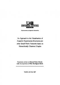
be to directly freeze the density matrix while letting atomic nuclei move 17 . However, when a non-orthogonal basis set is used, this may produce non-orthogonal molecular orbitals which might attract the system in configurations with actually higher potential energy. To address both issues, we propose a novel Block-Adaptive Quantum Mechanics (BAQM) approach, based on the DivideAnd-Conquer method and two new components. First, in order to decouple the computational complexity from the system’s size, we propose to adaptively simulate the nucleus degrees of freedom. In general, the nearsightedness principle 23 makes it possible to perform a fast incremental update of the electronic structure when only some atoms have moved 17,26,39,40 . In the Divide-And-Conquer approach 16 , the system is divided into nearly independent overlapping subsystems. In the context of a non self-consistent theory, when all atoms of a subsystem are frozen in space, both the Hamiltonian and its eigendecomposition are constant. To take advantage of this fact, we extend the approach we previously introduced for adaptive Cartesian mechanics coordinates 6 . Precisely, we freeze and unfreeze groups of atoms, according to the applied atomic forces and the system’s decomposition into overlapping subsystems. We call this first component Block-Adaptive Cartesian Mechanics. Second, to be able to deal with large subsystems for which diagonalization is the bottleneck, we propose to use an adaptively updated reduced basis which takes advantage of temporal coherence between successive eigendecomposition problems. For some methods, evaluating the Hamiltonian and overlap matrices may be computationally demanding. However, these computations are intrinsically parallel and can benefit from modern hardware architectures such as Graphics Processing Units (GPUs) 43 . Similarly, the computation of the density matrix has a cubic complexity in the number of basis functions, but dense matrix multiplications are memory-friendly 42,46 and can be efficiently handled on modern hierarchical-memory multicore architectures 13,45 . As a result, we have focused our efforts on the computation of molecular orbitals. A natural way to accelerate the resolution of many similar differential equations is to use a reduced basis approach 31 . This methodology has been applied in specific contexts for electronic structure calculation 12,29 . In this paper, we propose to use an adaptive reduced basis which is automatically updated during the simulation. We call this second component Adaptive Reduced-Basis Quantum Mechanics. We demonstrate that the BAQM approach may significantly speed-up energy minimization, as well as enable interactive quantum chemistry for large molecular systems. Figure 1 illustrates interactive virtual prototyping of a polyfluorene chain molecule.

Figure 1: Block-Adaptive Quantum Mechanics (BAQM) in SAMSON (Software for Adaptive Modeling and Simulation Of Nanosystems) 1 . In this example the system is divided into four subsystems. The energy is minimized continuously as the user edits the molecular system. At each time step, both the geometry and the electronic structure are incrementally and adaptively updated. Because the user pulls one atom (red arrow) in the left part of the system, the electronic structure is updated with the full basis for the leftmost subsystem (all atoms are red). In the neighboring subsystem, the electronic structure is updated according to a reduced-basis approximation (some carbons are black and some hydrogens are white). In the right part of the molecule, the user force does not have a sufficiently large impact, and atoms positions are frozen (all atoms are blue).

4

2

Overview

In general, adaptive approaches automatically focus computational resources on the most relevant parts of a problem. We use such an approach to maintain interactive rates while modeling chemical structures based on quantum chemistry principles. In this section, we provide an overview of our approach, and introduce its two main components: block-adaptive Cartesian mechanics, and adaptive reduced-basis quantum mechanics. For completeness, we first briefly recall the ASED-MO theory and the Divide-And-Conquer (D&C) technique. red We refer the reader to our previous publication 7 for more details about our ASED-MO D&C method.

2.1

The ASED-MO theory

In this paper, we used the ASED-MO theory 3 to test and validate our BAQM approach. In this theory, the electronic density function is split into two terms: a perfectly-following term (the electron density when atoms do not interact), and a non-perfectly-following term (corresponding to the bonds formation). This last term is computed based on the Extended Hückel Molecular Orbital theory (EHMO) 20 , a simple semi-empirical quantum chemistry method which approximates the Hamiltonian matrix terms as: Hµν = K

Iµ + Iν Sµν , 2

(6)

where Iµ is the ionization energy of the atomic orbital φµ , and K is the Wolfsberg-Helmholtz constant.

2.2

The Divide-And-Conquer (D&C) technique

red The D&C approach is attractive because of its efficiency (nearly perfect parallel scaling 32,35 ), simplicity for non-orthogonal basis sets, and accuracy 16,22,25,44,47,48 . There are three main steps in it: • Dividing the system

The original system S is first divided into M non-overlapping subsystems S1 , . . . , SM . Then, for each subsystem Si , an extended subsystem Si∗ is defined as the one containing all atoms from Si and those closer to these atoms than a certain distance cutoff.

• Computing each subsystem electronic structure independently

red A basis set is associated to each extended subsystem Si∗ (1 6 i 6 M ). The projection of the one-electron Schrödinger equation in redthis basis leads to the generalized eigenvalue problems:

Hi Ci = Si Ci Di , 1 6 i 6 M.

(7)

red Each local generalized eigenvalue problem (7) provides a set of molecular orbitals, which are then globally ranked according to their corresponding energies. We then populate these molecular orbitals until there are exactly N electrons in the system, as detailed in 7 . • Summing up the various contributions

red The occupied molecular orbitals determine the local density matrices Pi and energy-weighted density matrices Wi , from which the density matrix P and the energy-weighted density matrix W are obtained via a superposition scheme 7 . Once P and W have been obtained, the potential energy is expressed as E = Tr(HP )

(8)

and the gradient of the potential energy is approximated as: ∇x E =

XX µ

ν

Pµν ∇x Hµν −

5

XX µ

ν

Wµν ∇x Sµν .

(9)

2.3

Block-adaptive Cartesian mechanics

One possible adaptive approach to control the computational cost of each time step consists in reducing the number of nucleus degrees of freedom, to reduce the cost of updating the potential energy 6,34 . red In our ASED-MO D&C method 7 , the matrices Hi and Si involved in the eigenproblem (7) corresponding to subsystem Si are constant when all atoms in the extended subsystem Si∗ are frozen in space.

Consequently, we decide to adaptively freeze and unfreeze nuclei positions extended subsystem by extended subsystem. We

describe this approach in section “Block-adaptive Cartesian mechanics”.

2.4

Adaptive reduced-basis quantum mechanics

Block-adaptive Cartesian mechanics allows us to reduce the number of eigendecomposition problems that have to be solved at each time step. However, solving even just one of them may be too costly to achieve interactive rates. In order to accelerate molecular orbitals computation, we reduce the dimension of the basis in which the one-electron Schrödinger equation is projected. For any given subsystem, successive eigendecomposition problems are very similar, because atoms do not move significantly at each time step. Perturbation theory suggests that the subspace spanned by a cluster of eigenvectors might be rather insensitive to small perturbations 37 . To take advantage of this temporal coherence, we thus propose to use a reduced basis composed of low-energy eigenvectors computed at a previous time step. red To determine when the reduced basis should be updated, we use a simple distance measure between two generalized eigenvalue problems (7). We describe this approach in section “Adaptive reduced-basis quantum mechanic”.

2.5

Block-adaptive quantum mechanics

red Our BAQM approach combines the two components above to incrementally update the chemical structure of the molecular system at each time step. At the first time step (e.g. when the molecular system is loaded into memory), we compute the complete electronic structure of the system, as well as all forces applied on all atoms. This first step is used to initialize the BAQM process. Then, at each time step, we perform the following adaptive chemical structure update: • Block-adaptive Cartesian mechanics

(a) Adaptively freeze some extended subsystems. (b) For each active (unfrozen) atom, move along the force applied to it.

• Adaptive reduced-basis quantum mechanics

(a) For subsystems with mobile atoms, adaptively choose either a reduced-basis or a full-basis update of the molecular orbitals. red(b) For subsystems with mobile atoms, or for which some molecular orbital occupation’s number change, update the density matrices.

Section “The Block-Adaptive Quantum Mechanics algorithm” describes the BAQM algorithm in full detail.

3

Block-adaptive Cartesian mechanics

We now describe the block-adaptive Cartesian mechanics component, which consists in automatically freezing some positional degrees of freedom. As has been shown before, freezing atomic positions may accelerate geometry optimization of local defects 26,39 . Generally, these methods use a pre-defined active site, and only atoms in the active region are allowed to be mobile. In the context of interactive structural modeling, however, one cannot assume a pre-defined active site, since the user has the possibility to stress the system at any location. Therefore, to efficiently attract the system into low-energy regions, we need to efficiently choose the set of mobile atoms at each time step.

6

us approach of comparing To extend the atomic the previous force norms approach with of a certain comparing the atomic force norms wit We have recently introduced a novel adaptive algorithm which allows for interactive modeling with a reactive force field 6 .

extended subsystem force threshold, normwe f i⇤define for the anextended extended subsystem subsystem force Si⇤ . ofnorm f i⇤ for tothe extended su The key idea was to decide whether toSactivate or freeze an atom depending on the norm the force Sapplied it. Precisely,

⇤ smaller than a certain threshold value. Similarly, in quantum atom wasforce frozenPrecisely, if this norm by a thre ximumanatomic norm in Sfwas is the also maximum define a atomic threshold force value norm in Si⇤ . chemistry We alsomodels, define iS.i⇤ We

switching some positional degrees of freedom off, we may avoid updating some terms in the eigendecomposition problem (eq.

⇤ ⇤ . in ⇤ solve ⇤ , eigendecomposition ⇤ . When (2)). However, soon as af,S single changes the problem (eq. (7)), we have problem. Overview 2toa force Overview d 2to these force asnorms ffreeze which , .term . . , is fScompared When these norm force fnorms is afSnew . . . , f SM a force Sto 1 1 i M

It is thus very computationally attractive to freeze all atoms of an extended subsystem to avoid a new diagonalization.

⇤ ll atoms inextend the extended lower subsystem than ffreeze ,Sthen, arethe frozen allatomic atoms in space, innorms the extended subsystem Si⇤paradigm are frozen in sp To the previous approach of comparing force with athe certainthe threshold, an extended i paradigm In the general sense, the adaptive In consists the general in and automatically sense, adaptive fo- we define consists ∗ ∗ is the of maximum atomic force for the extended subsystem Scusing Precisely, fSparts subsystem force norm fS resources i . We also i . relevant cusing computational on the most computational theresources system. onnorm thein Smost mposition is not updated. corresponding On the eigendecomposition contrary, if there exists is not at updated. least On the contrary, if relevant there ex define a threshold value ffreeze , which is compared to these force norms fS , . . . , fS . When a force norm fS is lower than We use this approach to maintain interactive We rates use while this approach modeling to chemical maintain interactive rates whi ⇤ ffreeze , then, all atoms in the extended subsystem Si∗ are frozen in space, and the corresponding eigendecomposition is not orm larger than f one , we atom do with not choose a force to norm freeze larger all atoms than f of S , . we do not choose to freeze all freeze structures basedfreeze on quantum chemistry principles. structures In based this section, on iquantum we prochemistry principles. Ina updated. On the contrary, if there exists at least one atom with a force norm larger than ffreeze , we do not choose to freeze vide anatoms overview of our that approach and introduce an itscontain overview two main ofcomponents: our approach and its tw ⇤ all . Note that even ineven this case, though, Si∗vide may still frozen atoms, if it overlaps withintroduce some other, ase, though, Sofi⇤Si∗may Note still contain some in this frozen case, atoms, though, if itSsome may still contain some frozen atoms, i ioverlaps block-adaptive Cartesian mechanics, and adaptive block-adaptive reduced-basis Cartesian quantum mechanics, and adaptive red frozen subsystems. subsystems. withffreeze some The threshold value can other, either befrozen predefined by the user, or For automatically computed at timerecall step based mechanics. For completeness, we first recallsubsystems. the mechanics. Divide-And-Conquer completeness, (D&C) weeach first the on Dividethe system’s state. This value helps us control the computational cost a time step, one may directly control the To extend previous approach of force comparing forceof norms withsince a certain technique. technique. vious approach comparing thethreshold atomic norms withatomic a certain can eitherofthe be predefined The by the user, value or automatically f the can either computed be predefined by the user, or automaticall

reeze

∗ i

∗ i

∗ 1

∗ M

∗ i

number of performed diagonalizations. For fast energyfreeze minimization, we propose

we define force an extended subsystem extended force norm fSi⇤ for the Si⇤ . n threshold, extended subsystem norm fnorm subsystem Si⇤ .extendedSsubsystem Si⇤ for the force of the extended subsystem . Wenorm also define thresholdsub va force of the aextended

iThis value norm of⇤ the1the extended subsystem Si .force We define thres n the system’s state.atThis eachvalue time force step helpsbased us control on system’s computational state. helpsalso us control com norm of theathe exten f = max f . (10) 2.1 The (D&C) 2.1 The technique Divide-And-Conquer (D&C) te ⇤ atomic force norm in ⇤ is Divide-And-Conquer freeze S Precisely, f the maximum S . We also define a threshold value f , S M aximum atomici force norm f inMSi which . We also define a threshold value , i to 2these ⇤ , . . . , to ⇤ . Ws i=1..M fM compared subsystem force norms N N fM which compared ⇤ ,Sthese S fis force norms N . . . , Nt fis which is compared M which is compared to these subsystem S 1 M M 1 one may directly ⇤control cost of the a time number step, of since performed one may diagonalizations. directly control the number of performed diago ⇤ ⇤ ⇤ which is compared to these force norms f , . . . , f . When a force norm f is lower than ⇤ ⇤ norm NSnorm is lower fsteps. , technique then, atoms ofis a subsystem norm NSnorm ⇤subsystem Sforce SfM Sithree these force norms , . . . , afSM When norm is The lower than The technique is essentially Divide-And-Conquer composed isthe essentially com ThisDivide-And-Conquer scheme fisS1illustrated in. Figure 2. Mthan aa force subsystem NSi⇤ of isthan lower fMforce ,allthen, all the 1 a subsystem force Si⇤force i i ato ⇤corresponding extended subsystem arethefrozen spaceinand theand eigendec corresponding extended subsyst tion, we propose fast energy minimization, we fMextended , then, allsubsystem atoms inFor the extended subsystem Si⇤ the are frozen in propose space, and corresponding corresponding extended subsystem areinfrozen space the ei the are frozen in space, and corresponding • Dividing theSi system • Dividing the system corresponding extended is saved. one atom a oppositio forceBy position is saved. position is By saved. By opposition, ifatom it exists onewith atom ano f Step Step 1:it exists position is By saved. eigendecomposition iscontrary, notposition updated. On the contrary, ifopposition, there exists atifleast one with not updated. On the0: ifSthere exists at least one atom with The original system is first divided into non-overlapping The original system subsystems S is first divided intowith non-ove threshold1 larger than threshold fchoose we do case, than fMsubsystem. ,than weIndo freez larger fS ,, all weSfreeze do not the extended In this fthis , we do 1 larger M ,than Mnot ⇤ .extended Mnot ⇤to freeze S , . . . , S . Then, for each subsystem an extended , . . .of, the SSfreeze Then, Ssubsystem. each islarger S norm larger than f , we do not atoms . =5 Note thatfor even in subsystem 1 M i 1 Msubsystem i , an exte M ana fforce , we do not choose to freeze all atoms of S . Note that even in ⇤ ffreeze = f f (10) max f M =15 max i Si . freezei = Sii⇤ . can remark theSithat susbsytem can still contain some frozen atoms canthat remark the susbsytem contain some frozen ato remark that theSithat susbsytem can remark theas su i=1..M i=1..M 2 can defined as Scontaining all atoms from as well defined as those as containing closer to still atoms all atoms from as well as ⇤ 2 this case, though, may still contain some frozen atoms, if it overlaps with some other, may still contain somei frozen overlaps other, .cutoff. . . ,overlapping SMwith aresome overlapping .cutoff. . . ,overlapping SM are overlap S1 , atoms, . distance . . , SifSM2it, are S1 , . distance . . , SSM2 , are sub in Si than a certain insubsystems. Si than subsystems. a certain 30 The threshold 10 The threshold 4 10 frozen subsystems. fM either can besimply either simply by The predefined threshold value can2.be predefined by the user The threshold value fMvalue cant Mvalue d in Figure 2. This scheme is illustrated in fFigure • Solving each •at Solving each subsystem independently threshold value fsubsystem either beindependently predefined by computed the user, or automatically computed automatically at each time stepautomatically based on thecompute system M can automatically computed each time step based on the system state. automatically computed at eac e fM The can either be predefined by the user, or automatically computed Each extended subsystemhelps Si , us 1 6 i 6 M Each is associated extended with subsystem a vecS , 1 6 i 6 M is as tothe control the computational cost of control ai time as one m helps usastostep control the helps us to usstate. control the computational cost of a time step one may con helps us to the computa at each time stepstate. basedThis on the system’s This value helps us control the computational d on the torial system’s value helps control computational 3 6 1 4 2 10 subspace V in which the one-electron torial Schrödinger subspace equation V in which is the one-electron Sch 8 6 30 3the number 10 i8 i fast energy ofnumber diagonalization. For minimization, we the of number of the number ofcontrol diagonalization. For fastdiagonalizations. energy minimization, wediagonal propose the number diagonalization. a time step, since one may directly the of performed cecost one of may directly control the number of performed diagonalizations. projected, forming a generalized eigenvalue problem. projected, forming a generalized eigenvalue proble choose choose choose choose For fast energy minimization, we propose i i i i i i i ization, we propose fM =N(Smax NSi⇤H )/2 H C = S C D . fM = ( max C = S i C i D i . fM ⇤ )/2 (3) ∗ i

i=1..M

i=1..M i

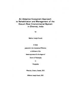
norm of the subsystem Si . Frozen We also define a thresholdFrozen value Atomic extended extended Mobile eigenvalu of the extended subsystem Si extended . Active We also define a threshold value 1scheme 1 of each Theforce solution local generalized eigenvalue The solution problem of (3) each deterlocal generalized This is illustrated in Figure 2. This scheme is illustrat S x x ⇤ f = max f . (10) M is S ⇤ . When fM = subsystem fSi⇤ .force (10)NS1⇤ ,2. fMthese which ismax compared tonorms these subsystem norms . . . , NThis This scheme in Figure scheme is illustrated in Fig ⇤ . subsystem system subsystem atom s compared to N When SM SM S i⇤ , . . . , iNforce i atom i=1..M 2Pillustrated 1 2 i=1..Mdensity mines the local matrix and energy mines weigthed the local density density matrix matrix P and energy wei ⇤ a subsystem force norm NSi is all lower fMof , then, all the atoms of the ⇤ m force norm the than atoms the i NSi is lower than fM , then, i W .corresponding Wspace . and the eigendecomin ngThis extended subsystem areextended frozen insubsystem space andare thefrozen eigendecomscheme is illustrated in Figure 2. ted in Figureposition 2. Snorm S S Step Step Step 1: 0: extended is saved. By opposition, if0: one atom with Sa isforce norm 2: Block-adaptive Cartesian mechanics. this example the system divided in saved. Figure By opposition, if it exists one with aexists force Sit In S S Step 0: atom Step 1: two Step 0: overlapping ∗ ∗ the various • subsystems Summing up contributions • Summing up the various contributions threshold fM =15 The subsystem. threshold fM=5fnorm. threshold M=15 The S1than andthe Sf2M , extended which havenot twofreeze atoms in each case, atom isone the atomic force larger , threshold we do thecommon. extended fM , we do not freeze subsystem. In this case,value oneindicatedInin this fM=15 threshold fMf=5 threshold M=15 value indicated in each subsystem is the subsystem force norm. The threshold value is automatically computed as half the In order to can compute the density P as Inand order the to energy-weighted compute P and can remark that the susbsytem canmatrix stillatoms contain some frozen atoms as∗ the the density matrix that the still some the valuesusbsytem of the maximum of thecontain subsystem force frozen norms. In step 0, f = 15 and, therefore, S is frozen. Consequently, only S2 S1 S1 i freezeS2 i S1 S 2 density Woverlapping from local matrices density and W matrix , a superposition W from theS1 local matrices P i and ∗ S1leftmost , . .matrix . , Satoms subsystems. are overlapping subsystems. S1 S1 S2 M areare the two mobile.the In step 1, ffreeze = 5S2 and,Ptherefore, the two rightmost 30 10 S1 is frozen. Consequently, only 4S2 30 10 1 threshold fP can simply predefined by user or P 4and are mobile. 30be 10 10 been ob scheme is Once and Weither have been scheme obtained, thethepotential Once 30 W have eshold atoms value fMThe canapplied. be eithervalue simply by 10 the user or is applied. Mpredefined automatically at on each stepstate. based system state. lly computed at is each timecomputed stepasbased thetime system fon energy expressed energy is expressed as fM M the helps us to control costmay of time step as one may control control the computational cost the of acomputational time E step as one ) 8acontrol (4) E 1 8 6 30 = Tr(HP 3 10 8 4 )8 2 30 3= Tr(HP 3 the number of diagonalization. For fast energy minimization, we propose to 3 1 4 of diagonalization. For fast energy minimization, we propose to 8 6 30 8 3 10 8 30 8 2 3 6 6 10 andchoose the gradient of the potential energy is approximated and the gradient as: of the potential energy is approx (6) fM = ( max NS ⇤ )/2 fM = ( max NSi⇤ )/2 (6)

⌅x E =i=1..M

i

Pµ⇥ ⌅x Hµ⇥

i=1..M

Wµ⇥ ⌅x S⌅ +⌅ = x Erep , P(5) µ⇥x E µ⇥ ⌅x Hµ⇥

Wµ⇥ ⌅x

Frozen extended Atomic Frozen Active This in FigureAtomic 2. µ ⇥ Si Active extended Si ⇥ µ ⇥ ⇥ Si e is illustrated in scheme Figure is 2.µillustrated x µ atom x S Frozen AtomicS Sisystem Active extended Si Frozen extended Mobile Atomic Active extended subsystem x subsystem system sub Si x x S x x S 7 system subsystem x subsystem system atom atom subsystem x x

4

Adaptive reduced-basis quantum mechanics

red In this section, we present the adaptive reduced-basis quantum mechanics component. Recall that, within any extended subsystem Si∗ , we want to solve a simplified problem by projecting problem (7), for the current time step, in a reduced basis

composed of low-energy eigenvectors that have been computed at a previous time step, to benefit from temporal coherence between successive eigenproblems. This is motivated by perturbation bound theory on the invariant subspace 37,38 . For clarity, we consider a system S with only one subsystem, and we first recall how the electronic structure problem (1)

may be projected to a reduced basis.

4.1

Electronic structure calculations in a reduced basis

red We consider two pairs of symmetric matrices: • (H ref , S ref ) the reference matrix pair for which an eigendecomposition is available. We denote by V ref the low-energy eigenvectors used as a reduced basis,

• (H , S ) the matrix pair related to the new system state. The matrix formulation of the new electronic structure problem in the reduced basis V ref is: H v C v = S v C v Dv ,

(11)

where H v and S v can be computed by matrix multiplication: H v = (V ref )T HV ref , S v = (V ref )T SV ref .

(12)

The diagonal matrix Dv contains the sorted eigenvalues (evi denotes the ith lowest eigenvalue). To compute forces, one could deal with the gradient of the reduced Hamiltonian H v and overlap matrix S v , since the resulting eigenvectors are expressed in basis V . However, these terms are complex and can lead to a quartic complexity for the forces expression. To compute forces in practice, we first express the eigenvectors in the full basis: red C n = V ref C v .

(13)

The resulting C n coefficients are the solution of the problem of finding the set of molecular orbitals minimizing the energy in the subspace generated by V . Then, the force formulation that expresses the variation of the energy calculated in the reduced basis (denoted E v ) by the atomic position is: ∇x E v =

XX µ

ν

v Pµν ∇x Hµν −

XX µ

ν

v Wµν ∇x Sµν ,

(14)

where P v is the density matrix i=1..N/2 v Pµν =

X

n n 2Cµi Cνi ,

(15)

n n 2evi Cµi Cνi ,

(16)

i

W v is the energy-weighted density matrix

i=1..N/2 v Wµν

=

X i

and C n is the matrix of the orthogonal molecular orbitals. One can remark that we do not speed-up the forces evaluation by the reduced-basis approach. The proof of equation (14) is presented in section “Appendix”. red

8

4.2

A temporal coherence measure

Let us use a simple distance ε between the two matrix pairs : q

ε=

||H − H ref ||2F + ||S − S ref ||2F ,

(17)

where ||.||F is the Frobenius norm. Then, the error in potential energy |E − E v | induced by the use of the reduced basis V

is asymptotically negligible compared to ε:

|E − E v | = O(ε2 )

(18)

The proof of this equation is presented in section “Appendix”. Consequently, we propose to use the distance ε as an indicator of the pertinence of using low-energy eigenvectors of (H

ref

, S ref ) to solve the new problem (H , S ), i.e. help us decide on the fly when to update the reduced basis by performing

a full-basis step (when ε becomes larger than a threshold value εM ).

4.3

Energy minimization with a reduced-basis approach

We recall that the main goal of our approach is to enable interactive geometry optimization, even for large systems. In general, one looks at this problem as the following energy minimization problem: min E(X), X

with X = {(xi )i=1..n } ∈ R3n , where E is the potential energy dependent on X, the nuclei positions. To understand why we can accelerate geometry optimization, we have to look at the problem as a minimization problem on both nucleus and electrons degrees of freedom. Let Z denote the vector space of the basis functions, then the problem reads as: N/2

min E(X, Ψ) = X,Ψ

X i=1

< ψi |H(X)|ψi >,

with X = {(xi )i=1..n } ∈ R3n , Ψ = {(ψi )i=1..N/2 } ∈ Z N/2 , subject to < ψi |S(X)|ψj >= δij , i, j = 1..N/2. We do not necessarily have to compute Ψ which minimizes E for each atomic position X (as is done when a complete diagonalization is performed). Our approach is to look for Ψ in a reduced basis, i.e., a Ψ which does not minimizes E for a given X. To guarantee convergence to local energy minima, we frequently update this reduced basis. Precisely, we perform at most kmax reduced basis steps between two full basis steps. Thus, unlike approaches which reduce the accuracy (by e.g. choosing a simpler model or decreasing the cutoff distance defining the extended subsystems size) to accelerate the simulation, our approach does not alter the final geometry of the molecule. In section “Results”, we demonstrate that the reduced basis can be used to accelerate interactive geometry optimization.

9

5

The Block-Adaptive Quantum Mechanics algorithm

In practice, we combine the two adaptive components described above in an algorithm which is now explicitly described. red

5.1

Algorithm initialization

At the very first step, a complete step is performed. ∀i ∈ 1..M , the generalized eigenvalue problem Hi Ci = Si Ci Di is

formulated and solved. We then populate the low-energy molecular orbitals until there are exactly N electrons in the system. We refer the reader to our previous work 7 for more details about the ASED-MO theory and our implementation of the D&C scheme.

5.2

Algorithm general step

We recall that ffreeze is a force threshold, εM is an eigendecomposition perturbation threshold and kmax the maximum number of reduced basis steps between full basis steps. fSi∗ is the maximum atomic force norm in Si∗ . (Hi , Si , Ci , Vi ) are respectively

the Hamiltonian, overlaps, eigenvectors, low-energy eigenvectors matrices of the extended subsytem Si∗ . (Hiref , Siref , Ciref , Viref )

are the reference matrices (for which the eigenproblem has been solved completely) of the extended subsytem Si∗ . We also

introduce ki a counter of the successive number of reduced basis steps in Si∗ . • Block-adaptive Cartesian mechanics – Update the threshold value ffreeze (e.g. ffreeze :=

1 max 2 i=1..M

fSi∗ ).

– ∀i ∈ 1..M , if fSi∗ < ffreeze , freeze the atoms of the extended subsytem Si∗ . – For each mobile atom, move along the force applied to it. • Incremental matrix computation: – ∀i ∈ 1..M , if Si∗ has some mobile atoms, compute the new Hamiltonian Hi and overlap matrix Si , as well as the

difference between them and the reference matrices Hiref and Siref from which we have deduced the reduced basis,

δHi and δSi . – ∀i ∈ 1..M , if Si∗ has some mobile atoms, compute εi := – Update the threshold value εM (e.g. εM :=

1 max 2 i=1..M

εi ).

p ||δHi ||2F + ||δSi ||2F .

• Adaptive reduced-basis quantum mechanics: ∀i ∈ 1..M , – If all atoms in Si∗ are frozen in space, keep the previous eigenvectors: Ci := Ciref . – Else, if ((0 < εi < εM ) and (ki < kmax )), perform a reduced-basis step: ∗ project: compute Hiv := (V ref )Ti Hi Viref and Siv := (V ref )TI Si Viref ,

∗ solve: compute a new set of molecular orbitals from eigenproblem (Hiv , Siv ),

∗ count: ki := ki + 1.

– Else, perform a full-basis step: ∗ solve: compute a new set of molecular orbitals from eigenproblem (Hi , Si ),

∗ update the reference eigenproblem: (Hiref , Siref , Ciref , Viref ) := (Hi , Si , Ci , Vi ), ∗ reset the counter: ki := 0.

• Finalize energy and forces computation – incremental molecular orbital occupation: ∗ for each extended subsystem Si∗ with new molecular orbitals, reset the density matrices (Pi := 0 and Wi := 0) and update the current total number of electrons in the system accordingly, 10

∗ globally sort unoccupied molecular orbitals by energy (remark that, in frozen subsystems, low-energy molecular orbitals are still occupied at this stage),

∗ populate low-energy molecular orbitals until there are exactly N electrons in the system (see note 1). – for each extended subsystem where the density matrix has been modified, incrementally update the atomic force of all atoms in the extended subsystem, (see note 2). – For each extended subsystem Si∗ with an atomic force change, update the maximum force norm of the subsystem fSi∗ .

Note 1 (incremental molecular orbitals occupation) During the incremental molecular orbital occupation stage, even the density matrices of frozen extended subsystems might change. Indeed, because the Fermi energy changes between two steps, it might happen that new molecular orbitals have to be occupied or that previously occupied molecular orbitals are not anymore populated with electrons. In this case, the density matrices can be efficiently updated via one or more rank-one matrix update. This is a rather rare event, however, when the time step size is small and there is high temporal coherence between successive steps, since the system’s energy is a continuous function of the atoms positions. Note 2 (incremental force update) Let us denote by fij the force acting on atom i due to the contribution of the extended subsystem Sj∗ to the density matrices P and W. Assuming fij = 0 when atom i does not belong to the extended subsystem Sj∗ , the total bonded force fi acting on atom i can be written:

fi =

X

fij .

(19)

j∈1..M

In our implementation, we incrementally update the forces, i.e. we only recompute the changing partial forces fij . Precisely, for each extended subsystem Sj∗ with density matrices changes, we first save each partial force before recomputing them: sji := fij . Then, the atomic force on atom i can be incrementally updated: fi := fi + fij − sji .

5.3

Choice of the threshold values

At least two options are possible for the choice of the thresholds ffreeze and εM . The simplest choice is to predefine these values. In this case, the system will not relax completely (since some atoms with non-zero applied forces will not move). However, this approach is very powerful when the user is prototyping a new system and does not need the full accuracy of the quantum chemistry model. In this mode, an adaptive minimization step is performed only when the modeler detects that large forces are applied or that an important perturbation in the eigendecomposition problem appeared. Two videos in the Supporting Material illustrates adaptive quantum chemistry modeling. The second option is to automatically choose the thresholds based on the system’s state. Let K denote a user-defined constant. We may choose ffreeze = (maxi=1..M fSi∗ )/K and εM = (maxi=1..M εi )/K. Consequently the computational resources will be focused on the most mobile atoms and on the most perturbed eigendecomposition problems. For interactive quantum chemistry modeling, one may also compute the threshold values to allow only N1 subsystems with mobile atoms and N2 subsystems with diagonalisation such that the time cost of each step is well controlled. red Two options are also possible for kmax . In practice, for interactive quantum chemistry, we choose a value kmax = 100. However, in section “Results”, we show that kmax can be optimized for a faster energy minimization.

11

6

Results

We now present results of our block-adaptive quantum mechanics algorithm for the ASED-MO level of theory. redIn this paper, we focus on the BAQM approach performance and we refer the reader to our previous work 7 about our ASED-MO D&C approach for more details about its accuracy and efficiency. We have used C++ as the main programming language. We have also used the highly optimized multithreaded Intel Math Kernel Library 21 to solve the generalized eigenvalue problems and to perform all the linear algebra operations. The tests have been performed on two different computers. Computer 1 is a desktop computer with two 2.67 GHz quad-core processors and 4GB of RAM, running a 32-bit Linux Fedora operating system. Computer 2 is a desktop computer with two 2.33 GHz quad-core processor and 4GB of RAM, running a 32-bit Linux Fedora operating system.

6.1

Reduced-basis molecular orbital computations

In this section, we compare full-basis and reduced-basis molecular orbitals computations. Computer 1 was used in this test. We recall that, for fast steps, we have to perform the linear algebra operations H v = B T HB, S v = B T SB, solve the eigendecomposition H v C v = S v C v E v , and perform C n = BC v . We also compare this scheme with a simpler Sorthogonalization. Indeed, an S-orthogonalization of the molecular orbitals can be used when the system S contains only

one subsystem and the reduced basis dimension coincides with the number of occupied molecular orbitals. In this case, any S-orthogonal basis of the occupied subspace results in the same energy, and is a better choice if one is not interested in the molecular orbitals (eigenvectors and eigenvalues) themselves. Figure 3 presents timings averaged over 100 evaluations for different matrix sizes (the method does not depend on the matrix elements). All curves demonstrate a cubic behavior. With the implementation presented in the appendix, the simple orthogonalization of 50% of the previous eigenvectors is about one order of magnitude faster than the full basis approach. Therefore, adaptive reduced-basis quantum mechanics allows for interactive rates with larger subsystems.

Figure 3: Timings of reduced-basis molecular orbitals computations with different basis dimensions. The eigendecomposition problem is projected in a basis containing respectively 100%, 80%, 70%, 60% or 50% of the low energy eigenvectors of a previously solved problem.

12

6.2

Energy minimization with the adaptive reduced-basis approach

We recall that, in our approach, the main goal is to provide interactive and efficient geometry optimization. During an interactive modeling session, on-the-fly geometry optimization assists the user by continuously attracting the system into lower energy states. The previous section demonstrates that using a reduced basis leads to faster steps, which allows for interactive rates with larger subsystems. We now demonstrate the relevance of the adaptive reduced-basis approach for accelerating energy minimization. In interactive geometry optimization, sophisticated methods such as quasi-newton or conjugate gradient may not be appropriate since each minimization step may require several forces and potential energy evaluations, making it more difficult to achieve interactive rates with large systems. Our approach is simply to use a steepest descent method with a constant time step size to have a smooth attraction of the system into a local minimum. red For four structures (fullerene, polyflurorene, nanotube and graphene) presented in Figure 4, we optimized the geometry and obtained the global minimum of the potential energy. Then, we repeated the optimization with the adaptive reducedbasis approach and stopped the energy minimization when the potential energy E was close enough to the global minimum −3 0 energy E0 (| E−E ). In these tests, we did not use εM to decide when to switch, but simply alternated between E0 | < 10

kmax reduced-basis steps and one full-basis step. The reduced bases were always composed of 50% of the previously solved eigendecompositon problem so that, since the dimension of the reduced basis coincided with the number of molecular orbitals to be computed, we simply performed an orthogonalization of the molecular orbitals. These tests were performed using computer 1. Figure 5 presents the different speed-ups as a function of kmax , the number of reduced basis steps between each full basis step. One can see that larger systems appear to benefit more from our approach, as molecular orbitals computation largely dominates the cost of a simulation step. Geometry optimizations that include bond formations (fullerene and nanotube tests) benefit less from our approach. Remark that, when kmax is large, our approach slows down energy minimization (the speed-up is smaller than 1).

6.3

Energy minimization with the Block-Adaptive Quantum Mechanics (BAQM) approach

Here, we demonstrate how the BAQM algorithm (section “The Block-Adaptive Quantum Mechanics algorithm”) may be used to accelerate the geometry optimization of a locally deformed graphane sheet of 1556 atoms. In this structure, each carbon atom is bound to one hydrogen atom, explaining the potential role of graphane as an hydrogen storage medium 36 . Stable graphane structures were first theoretically predicted and then experimentally realized. The lowest potential energy structure is achieved when hydrogen atoms are attached to the graphane sheet in an alternating pattern (up and down). An important problem is to understand the role of H–frustration 27 . In this minimization test, one hydrogen bond was flipped in such a way that two hydrogen atoms became frustrated, and the geometry of the graphane sheet had to be relaxed. We used 64 subsystems and a cut-off of 6 Å to define the extended subsystems. The tests were performed on computer 2. Figure 6 shows the Root-Mean-Square-Deviation (RMSD) to the optimized structure as a function of wall-clock time while energy minimization was performed and reports the resulting speed-ups. Energy minimization was stopped when a 0.01 RMSD was reached. The BAQM approach allows for a speed-up of more than 20 by choosing the threshold value ffreeze automatically computed by ffreeze = (maxi=1..M fSi∗ )/2 and by updating the reduced basis every 6 steps (i.e. for kmax = 5, without using εM ). The reduced basis sets were composed of 50% of the previously solved eigendecomposition problem (orthogonalization was not used because we needed to access each eigenvalue individually in the D&C scheme). The adaptive reduced-basis approach itself allowed us to speed-up minimization by a factor of 1.4. The block-adaptive cartesian mechanics allowed for an important speed-up of 16, since only some atoms had to be moved to relax the structure. We note that the total speed-up allowed by the BAQM approach was approximately the multiplication of these two speed-ups, which shows that the two components developed in this paper combine well.

13

a

b

c

d

Figure 4: redThe four structures considered in the energy minimization benchmarks. (a) is a buckminster fullerene (C60 ), (b) is a graphene sheet (C216 ), (c) is a polyfluorene molecule (C90 H72 ) and (d) is a carbone nanotube (C200 ). Remark that geometry optimization of molecules (a) and (d) requires bonds formation. The white surface is an isosurface of the electron density.

14

4

4 Graphene

Polyfluorene 3 Speed-up

Speed-up

3

2

1

2

1

0

0 0

100 200 300 Number of fast steps (k max)

400

0

4

200 400 600 800 Number of fast steps (k max)

4 Nanotube

Fullerene 3 Speed-up

3 Speed-up

1,000

2

1

2

1

0

0 0

20 40 60 80 Number of fast steps (k max)

100

0

10

20 30 40 Number of fast steps (k max)

50

Figure 5: redDifferent speed-ups for convergence to global minima are presented. The number in the abscissa represents Nanotube (C200) kmax , the number of reduced basis steps between each full basis step (reduced basis update).

15

Figure 6: Performance of the block-adaptive divide-and-conquer approach for energy minimization. The figure plots the Root-Mean-Square Deviation (RMSD) to the minimized structure of a graphane sheet as a function of wall-clock time during energy minimization. Geometry optimization is stopped when the RMSD is smaller than 0.01 Å. In this case, our block-adaptive D&C approach allows for an important speed-up. Speed-ups of the different adaptive approaches are indicated into brackets in the legend.

16

6.4

Interactive quantum chemistry demonstration

For many systems, our approach is sufficiently efficient to enable interactive quantum chemistry simulations on a multicore desktop computer. In the Supporting Material, we present two videos demonstrating interactive quantum chemistry modeling in SAMSON 1 , the software being developed in our group. We used computer 1. In these examples, the user interactively edits the systems by pulling on atoms. The imposed atomic displacement is proportional to the distance between the selected atom and the position of the mouse pointer. • Interactive quantum chemistry with a large subsystem: the user loads a carbon nanotube of 120 atoms treated with the ASED-MO theory with 480 basis elements and only one subsystem. For this system, the classical approach

allows only 5 energy and forces computations per second. Thanks to the reduced basis approach, 20 energy and forces evaluations per second can be achieved and the user may interactively prototype the system. In the reduced basis approach, bonds may break and re-form, however, the reduced basis, which has been deduced from the electronic structure of the initial geometry of the system, prevents the system from creating new bonds. To overcome this limitation, the user activates the Adaptive Reduced-Basis Quantum Mechanics approach. Then, in this example, the user is able to intuitively edit the system and explore different chemical structures. Figure 7 illustrates this interactive session. • Interactive quantum chemistry with a large system: the user loads a graphane sheet of 1556 atoms treated with

the ASED-MO divide-and-conquer approach. 64 subsystems are used and a cut-off of 4 Å for the buffer zone is chosen to achieve interactivity with our block-adaptive approach. The user is able to study the impact on the geometry of the structure when the state of a carbon-hydrogen chemical bond is changed. The bond can be broken and reformed on the other side of the graphane sheet. The block-adaptive quantum mechanics approach allows the user to interactively prototype the structure with each time step being approximately one order of magnitude faster. Figure 8 illustrates this interactive session. The BAQM approach also allows us to efficiently access different optimized configurations as illustrated in Figure 6.

17

a

b

c

Figure 7: Interactive modeling session. The user selects a group of atoms (atoms in blue) and splits the carbon nanotube into two parts (a). Then, the user pulls on a carbon atom to break a bond (b) and designs a new chemical structure (c). The user force is displayed by a red arrow.

a

b

c

Figure 8: Interactive modeling session. The user loads a graphane sheet composed of 1556 atoms (a). The user selects a hydrogen atom and applies a force (b). The user succeeds to break the bond (c). The user force is displayed by a red arrow.

18

7

Conclusion

In this paper, we demonstrate that interactive quantum chemistry simulation is feasible for rather large systems in the framework of the ASED-MO theory and the Divide-And-Conquer (D&C) technique. The proposed Block-Adaptive Quantum Mechanics (BAQM) approach allows for interactive rates with larger systems and larger subsystems than in the original scheme. We reduced the percentage of the time spent in the diagonalization routine. As a result, optimization and multithreading on the rest of the computations can significantly improve the speed of a simulation, so that interactive quantum chemistry should be feasible for systems up to few thousands of atoms in the near future thanks to technological progress. To achieve these results, we developed two adaptive approaches in which nuclei positions as well as electronic degrees of freedom can be constrained on the fly to control the simulation cost. First, we presented a block-adaptive Cartesian mechanics approach, in which nuclei may be frozen in space in groups, which allows us to deal with large systems. Second, we proposed to use a reduced basis set composed of some of the low-energy eigenvectors of a previous time step to accelerate the molecular orbital computations in large subsystems. The reduced basis is adaptively updated. We demonstrated that these approaches may accelerate geometry optimization. Indeed, each step is solved significantly faster by constraining some nuclei and electrons, and, by focusing computational resources on the most mobile atoms, we obtain a faster potential energy descent. The presented method is general, and should be applicable to many quantum chemistry models. We would like to determine whether it might be useful to accelerate geometry optimization with self-consistent models, and/or large basis sets such as real space grids 9 , plane waves 24 or wavelets 18 . The idea of adaptively constraining the degrees of freedom in Cartesian coordinate 6 can also be used to accelerate phasespace sampling in the framework of the Adaptively Restrained Particle Simulations (ARPS) algorithm 4 . We would like to investigate whether the adaptive reduced basis approach may be efficiently combined to ARPS to efficiently compute statistical properties with quantum chemistry models.

8 8.1

Appendix Forces expression in a reduced basis approach

Let us prove the force formulation presented in section “Electronic structure calculations in a reduced basis”. Theorem: The gradient with respect to an atomic position x of the potential energy computed with a reduced basis is: ∇x E v =

XX µ

ν

Proof: ∇x E v = ∇ x then, ∇x E v =

X i

however,

and

X i

X

2(∇x Civ )T H v Civ +

As Civ are eigenvectors, we have: ∇x E v =

v Pµν ∇x Hµν −

i

2evi = ∇x

X

XX µ

X

ν

v Wµν ∇x Sµν ,

2(Civ )T H v Civ ,

(20)

(21)

i

2(Civ )T (∇x H v )Civ +

i

X

2(Civ )T H v (∇x Civ ).

(22)

i

  X 2(Civ )T (∇x H v )Civ , 2evi (∇x Civ )T S v Civ + (S v Civ )T (∇x Civ ) +

(23)

i


(∇x Civ )T S v Civ + (Civ )T S v (∇x Civ ) = ∇x Civ )T S v Civ − (Civ )T (∇x S v )Civ ,   ∇x (Civ )T S v Civ = ∇x 1 = 0. 19

(24)

(25)

As a result, ∇x E v = −

X i

We can develop the terms:

  X 2evi (BCiv )T ∇x S(BCiv ) + (BCiv )T (∇x H)BCiv .

(BCiv )T ∇x S(BCiv ) = (Cin )T ∇x S(Cin ) =

XX

n n Cµi Cνi ∇x Sµν ,

(27)

(BCiv )T ∇x H(BCiv ) = (Cin )T ∇x H(Cin ) =

XX

n n Cµi Cνi ∇x Hµν .

(28)

Finally, ∇x E v =

8.2

(26)

i

XX µ

ν

v Pµν ∇x Hµν −

µ

ν

µ

ν

XX µ

ν

v Wµν ∇x Sµν

(29)

An order-one correction

Let us consider two pairs of symmetric matrices: • (H ref , S ref ) for which an eigendecomposition is available, we denote V the low-energy eigenvectors and W the remaining N 2.

eigenvectors. We assume that the rank of V is larger than

• (H , S ) related to the new system state. Let us define a simple distance between the two matrix pairs ε as: ε=

q

||H − H ref ||2F + ||S − S ref ||2F ,

(30)

Let us show that projecting the new problem in the previous low-energy eigenvectors results in an order-one correction of the system’s potential energy. For clarity, we first introduce four lemma. • Lemma 1:

Let H r and S r denote the new Hamiltonian and overlap matrices expressed in the old eigenvector basis Z = (V, W ): H r = Z T H Z, S r = Z T S Z.

Precisely: Hv

H v−w

(H v−w )T

Hw

r

H =

!

Sv

S v−w

(S v−w )T

Sw

r

, S =

(31) !

(32)

where H v = V T H V, S v = V T S V,

(33)

H w = W T H W, S w = W T S W,

(34)

H v−w = V T H W, S v−w = V T S W.

(35)

The eigenvalues of (H r , S r ) are also eigenvalues of (H , S ).

• Lemma 2:

Let H p and S p denote the matrices of the approximate Hamiltonian by neglecting H v−w : p

H =

Hv

0

0

Hw

!

20

p

, S =

Sv

0

0

Sw

!

.

(36)

When the largest eigenvalue of the matrix pair (H v , S v ) is lower than the lowest eigenvalue of the matrix pair (H w , S w ), the sum of the

N 2

lowest eigenvalues of (H p , S p ) is the sum of the

N 2

lowest eigenvalues of (H v , S v ).

• Lemma 3:

Let H a and S a denote the matrices of the approximate Hamiltonian by neglecting H v−w expressed in the full basis: H a = Z −T H p Z −1 , S a = Z −T S p Z −1 .

(37)

The eigenvalues of (H a ,S a ) are those of (H p ,S p ) and we can state that: q ||H a − H ref ||2F + ||S a − S ref ||2F = O(ε).

(38)

||H ref − H ||F = O(ε), ||S ref − S ||F = O(ε)

(39)

||Z T (H ref − H )Z||F = O(ε), ||Z T (S ref − S )Z||F = O(ε)

(40)

||Dref − H r ||F = O(ε), ||I − S r ||F = O(ε),

(41)

Proof: As

and Z is constant, we have

which can be rewritten as

where Dref denotes the diagonal matrix of the ordered eigenvalues of the matrix pair (H ref , S ref ). Since both (block-)diagonal elements of H r − H p and S r − S p are zero, we have: ||H p − H r ||F ≤ ||Dref − H r ||F , ||S p − S r ||F ≤ ||I − S r ||F .

(42)

Consequently, from equations (41) and (42), we have ||H p − H r ||F = O(ε), ||S p − S r ||F = O(ε).

(43)

||Z −T H p Z −1 − Z −T H r Z −1 ||F = O(ε), ||Z −T S p Z −1 − Z −T S r Z −1 ||F = O(ε),

(44)

Since, again, Z is constant,

which can be rewritten as ||H a − H ||F = O(ε), ||S a − S ||F = O(ε).

(45)

From equations (39) and (45), we can conclude that ||H a − H ref ||F = O(ε), ||S a − S ref ||F = O(ε).

(46)

• Lemma 4:

Let ei denote the ith lowest eigenvalue of (H , S ) and epi the ith lowest eigenvalue of (H p , S p ), we have |ei − epi | = O(ε2 )

(47)

Proof: One can apply eigenvalue perturbation theory with the matrix pairs (H , S ) and (H ref , S ref ). In the limit of

21

small perturbations, the order of the eigenvalues is not changed and we can state: 2 ei = eold + ziT (H − eold i i S )zi + O(ε ).

(48)

where zi is the ith eigenvector of (H ref , S ref ). By definition of (H r , S r ), we can rewrite equation (48) r 2 ei = eold + Hiir − eold i i Sii + O(ε ).

(49)


One can apply eigenvalue perturbation theory with the matrix pairs H a , S a and (H ref , S ref ). In view of lemma 3, this may be written as

which is simply


−T p −1 zi + O(ε2 ). epi = eold + ziT Z −T H p Z −1 − eold S Z i i Z p 2 + Hiip − eold epi = eold i i Sii + O(ε ).

(50)

(51)

p r = Sii , we can state that Since Hiip = Hiir and Sii

|ei − epi | = O(ε2 ).

(52)

Theorem: The potential energy error |E − E v | induced by the use of the reduced basis V is asymptotically negligible compared to ε:

|E − E v | = O(ε2 ).

(53)

Proof: In view of lemma 1, the potential energy E is the sum of the lowest eigenvalues of (H r , S r ): E=

X

2ei ,

(54)

i=1.. N 2

In the limit of small ε, the largest eigenvalue of the matrix pair (H v , S v ) is lower than the lowest eigenvalue of the matrix pair (H w , S w ). Thus, in view of lemma 2, the reduced-basis potential energy E v is the sum of the lowest eigenvalues of (H p , S p ): Ev =

X

2evi =

i=1.. N 2

X

2epi ,

(55)

i=1.. N 2

In the limit of small ε, lemma 3 implies that we can write the potential energy error |E − E v | induced by the use of a

reduced basis as:

|E − E v | =

X

i=1.. N 2

2(ei − epi ) =

X

2(O(ε2 )) = O(ε2 ),

(56)

i=1.. N 2

which shows that projecting the new problem (H , S ) in the previous low-energy eigenvectors results in an order-one correction of the system’s potential energy.

8.3

A multithreaded orthogonalization solver

In general, orthogonalization has a cubic scaling. However, it can be efficiently performed on multicore architecture 2,10,11,28 . Unfortunately, we are considering S-orthogonalization and we had to implement an orthogonalization algorithm for this specific case. We chose the modified Gram-Schmidt algorithm 19 . As a result, we designed it in such a way that for our system’s sizes the algorithm provides a good speed-up when using the multithreaded variant of the code using OpenMP 14 . Let N denote the number of occupied molecular orbital, S – the overlap matrix, and B – the reduced basis.

22

Algorithm 1 S-orthogonalisation solver Require: A matrix S and a matrix B with the vectors to S-orthogonalize. Ensure: B contains S-orthogonal vectors. 1: 2: 3: 4: 5: 6: 7: 8: 9: 10: 11: 12:

SB ← S ∗ B for i = 1 → Npdo norm ← B(:, i)T ∗ SB(:, i) 1 B(:, i) ← norm ∗ B(:, i) {The vector B(:, i) is now S-normalized} 1 SB(:, i) ← norm ∗ SB(:, i) #Loop using multithreading for j = i + p1 → N do x ← B(:, i)T ∗ SB(:, j) B(:, j) ← B(:, j) − x ∗ B(:, i) {B(:, i) and B(:, j) are now S-orthogonal} SB(:, j) ← SB(:, j) − x ∗ SB(:, i) end for end for

References 1. SAMSON (Software for Adaptive Modeling and Simulation Of Nanosystems). NANO-D. http://nano-d.inrialpes.fr/. 2. E. Agullo, J. Dongarra, R. Nath, and S. Tomov. A fully empirical autotuned dense QR factorization for multicore architectures. Technical report, Technical Report 242, LAPACK Working Note, 2011. 3. A. B Anderson. Electron density distribution functions and the ASED-MO theory. International Journal of Quantum Chemistry, 49(5):581–589, 1994. 4. S. Artemova and S Redon. ARPS: Adaptively Restrained Particle Simulations. To be published, 2012. 5. P. Bientinesi, I.S. Dhillon, and R.A. Van De Geijn. A parallel eigensolver for dense symmetric matrices based on multiple relatively robust representations. SIAM Journal on Scientific Computing, 27(1):43–66, 2006. 6. M. Bosson, S. Grudinin, X. Bouju, and S. Redon. Interactive physically-based structural modeling of hydrocarbon systems. Journal of Computational Physics, 2011. 7. M. Bosson, C. Richard, A. Plet, S. Grudinin, and S. Redon. Interactive quantum chemistry: A divide-and-conquer ASED-MO method. Journal of Computational Chemistry, 2012. 8. Elena Breitmoser and Andrew G. Sunderland.

A performance study of the PLAPACK and SCALA-

PACK eigensolvers on hpcx for the standard problem. Tethnical Report from the HPCx Consortium. http://www.hpcx.ac.uk/research/hpc/hpcxtr0406.pdf, 2004. 9. EL Briggs, DJ Sullivan, and J. Bernholc. Real-space multigrid-based approach to large-scale electronic structure calculations. Physical Review B, 54(20):14362, 1996. 10. A. Buttari, J. Langou, J. Kurzak, and J. Dongarra. Parallel tiled qr factorization for multicore architectures. Concurrency and Computation: Practice and Experience, 20(13):1573–1590, 2008. 11. A. Buttari, J. Langou, J. Kurzak, and J. Dongarra. A class of parallel tiled linear algebra algorithms for multicore architectures. Parallel Computing, 35(1):38–53, 2009. 12. E. Cances, C. Le Bris, NC Nguyen, Y. Maday, A.T. Patera, and GSH Pau. Feasibility and competitiveness of a reduced basis approach for rapid electronic structure calculations in quantum chemistry. In Proceedings of the Workshop for Highdimensional Partial Differential Equations in Science and Engineering (Montreal), 2007. 13. E. Chan, E.S. Quintana-Orti, G. Quintana-Orti, and R. Van De Geijn. Supermatrix out-of-order scheduling of matrix operations for smp and multi-core architectures. In Proceedings of the nineteenth annual ACM symposium on Parallel algorithms and architectures, pages 116–125. ACM, 2007. 23

14. R. Chandra. Parallel programming in OpenMP. Morgan Kaufmann, 2001. 15. C.J. Cramer. Essentials of computational chemistry: theories and models. John Wiley & Sons Inc, 2004. 16. S.L. Dixon and K.M. Merz Jr. Semiempirical molecular orbital calculations with linear system size scaling. Journal of Chemical Physics, 104(17):6643–6649, 1996. 17. M.D. Ermolaeva, A. van der Vaart, and K.M. Merz Jr. Implementation and testing of a frozen density matrix-divide and conquer algorithm. The Journal of Physical Chemistry A, 103(12):1868–1875, 1999. 18. L. Genovese, A. Neelov, S. Goedecker, T. Deutsch, S.A. Ghasemi, A. Willand, D. Caliste, O. Zilberberg, M. Rayson, A. Bergman, et al. Daubechies wavelets as a basis set for density functional pseudopotential calculations. The Journal of chemical physics, 129:014109, 2008. 19. G.H. Golub and C.F. Van Loan. Matrix computations, volume 3. Johns Hopkins Univ. Press, 1996. 20. R. Hoffmann. An extended Hückel theory. I. Hydrocarbons. Journal of Chemical Physics, 39(6):1397–1412, 1963. 21. Intel. Math kernel library.www.intel.com/software/products/mkl. 22. M. Kobayashi and H. Nakai. Divide-and-conquer approaches to quantum chemistry: Theory and implementation. LinearScaling Techniques in Computational Chemistry and Physics, pages 97–127, 2011. 23. W. Kohn. Density functional and density matrix method scaling linearly with the number of atoms. Phys. Rev. Lett., 76(17):3168–3171, Apr 1996. 24. G. Kresse and J. Furthmüller. Efficiency of ab-initio total energy calculations for metals and semiconductors using a plane-wave basis set. Computational Materials Science, 6(1):15–50, 1996. 25. T. S Lee, J. P Lewis, and W. Yang. Linear-scaling quantum mechanical calculations of biological molecules: The divide-and-conquer approach. Computational Materials Science, 12(3):259–277, 1998. 26. Tai-Sung Lee and Weitao Yang. Frozen density matrix approach for electronic structure calculations. International Journal of Quantum Chemistry, 69(3):397–404, 1998. 27. S.B. Legoas, P.A.S. Autreto, M.Z.S. Flores, and D.S. Galvao. Graphene to graphane: the role of H frustration in lattice contraction. Arxiv preprint arXiv:0903.0278, 2009. 28. L. Liu, Z. Li, and A.H. Sameh. Analyzing memory access intensity in parallel programs on multicore. In Proceedings of the 22nd annual international conference on Supercomputing, pages 359–367. ACM, 2008. 29. Y. Maday and U. Razafison. A reduced basis method applied to the Restricted Hartree–Fock equations. Comptes Rendus Mathematique, 346(3):243–248, 2008. 30. R.S. Mulliken. Spectroscopy, molecular orbitals, and chemical bonding. Nobel Lecture, December 12, 1966. 31. A.K. Noor and J.M. Peters. Reduced basis technique for nonlinear analysis of structures. In Structures, Structural Dynamics, and Materials Conference, 20 th, St. Louis, Mo, pages 116–126, 1979. 32. W Pan, T S Lee, and W T Yang. Parallel implementation of divide-and-conquer semiempirical quantum chemistry calculations. Journal of Computational Chemistry, 19(9):1101–1109, 1998. 33. M. J. Rayson and P. R. Briddon. Rapid iterative method for electronic-structure eigenproblems using localised basis functions. Computer Physics Communications, 178(2):128–134, January 2008. 34. R. Rossi, M. Isorce, S. Morin, J. Flocard, K. Arumugam, S. Crouzy, M. Vivaudou, and S. Redon. Adaptive torsion-angle quasi-statics: a general simulation method with applications to protein structure analysis and design. Bioinformatics, 23(13):i408–i417, 2007. 24

35. F. Shimojo, R.K. Kalia, A. Nakano, and P. Vashishta. Divide-and-conquer density functional theory on hierarchical real-space grids: Parallel implementation and applications. Physical Review B, 77(8):085103, 2008. 36. J.O. Sofo, A.S. Chaudhari, and G.D. Barber.

Graphane: A two-dimensional hydrocarbon.

Physical Review B,

75(15):153401, 2007. 37. G.W. Stewart. Pertubation bounds for the definite generalized eigenvalue problem. Linear algebra and its applications, 23:69–85, 1979. 38. G.W. Stewart and J. Sun. Matrix perturbation theory, volume 175. Academic press San Diego, CA, 1990. 39. J.J.P. Stewart. Application of localized molecular orbitals to the solution of semiempirical self-consistent field equations. International journal of quantum chemistry, 58(2):133–146, 1996. 40. P.R. Surján, D. Kohalmi, Z. Rolik, and Á. Szabados.

Frozen localized molecular orbitals in electron correlation

calculations-exploiting the hartree-fock density matrix. Chemical Physics Letters, 450(4-6):400–403, 2008. 41. H. Sutter. The free lunch is over: A fundamental turn toward concurrency in software. Dr. Dobb’s Journal, 30(3):202–210, 2005. 42. M. Thottethodi, S. Chatterjee, and A.R. Lebeck. Tuning Strassen’s matrix multiplication for memory efficiency. In Proceedings of the 1998 ACM/IEEE conference on Supercomputing (CDROM), pages 1–14. IEEE Computer Society, 1998. 43. I.S. Ufimtsev and T.J. Martínez. Quantum chemistry on graphical processing units. 1. strategies for two-electron integral evaluation. Journal of Chemical Theory and Computation, 4(2):222–231, 2008. 44. Arjan Van Der Vaart, Dimas SuÃąrez, and Kenneth M Merz. Critical assessment of the performance of the semiempirical divide and conquer method for single point calculations and geometry optimizations of large chemical systems. Journal of Chemical Physics, 113(23):10512–10523, 2000. 45. V. Volkov and J.W. Demmel. Benchmarking gpus to tune dense linear algebra. In High Performance Computing, Networking, Storage and Analysis, 2008. SC 2008. International Conference for, pages 1–11. IEEE, 2008. 46. R.C. Whaley, A. Petitet, and J. Dongarra. Automated empirical optimizations of software and the ATLAS project. Parallel Computing, 27(1-2):3–35, 2001. 47. W. Yang and T.S. Lee. A density-matrix divide-and-conquer approach for electronic structure calculations of large molecules. Journal of Chemical Physics, 103(13):5674–5678, 1995. 48. R. Zalesny, M.G. Papadopoulos, P.G. Mezey, and J. Leszczynski. Linear-scaling techniques in computational chemistry and physics: Methods and applications. Challenges and Advances in Computational Chemistry and Physics (13), 2011.

25