An Adaptive Meta-classifier for Text Documents Radu G. Creţulescu, Daniel I. Morariu, Lucian N. Vinţan Faculty of Engineering, “Lucian Blaga” University of Sibiu, Computer Science Department, E. Cioran Street, No. 4, 550025 Sibiu, ROMANIA, {radu.kretzulescu, daniel.morariu, lucian.vintan}@ulbsibiu.ro
and Irina D. Coman Center for Applied Software Engineering at the Free University of Bozen-Bolzano, Piazza Universita 1, 39100, Bolzano, Italy
[email protected] ABSTRACT In this paper we investigated a way to create a new adaptive metaclassifier for classifying text documents in order to increase the classification accuracy. During the first processing phase (preclassification) the meta-classifier uses a non-adaptive selector. The role of this selector is to implement a data transformation from a large space representation of the documents (in our case vectors having 1309 words) into a much smaller space representation, based on the input data categories (in our case there are 16 categories). This transposition method is based on the categories in which the input data might be classified (Reuter’s classification) and it is using SVM and Bayes type classification algorithms. In the second phase (classification) we use a feed-forward neural network based on the back-propagation learning method. We chose a neural network architecture which contains one hidden layer of units with sigmoid activation function, where each unit from each layer is connected with all units of the previous layer. The experimental results have showed that using this adaptive algorithm, classification accuracy can be significantly improved. For Reuters2000 text documents we obtained classification accuracy up to 99.74%.
Keywords: Meta-classification, Back propagation Networks and Text Document Classification 1. INTRODUCTION Storing and retrieving information was and remains a concern for mankind since it began reaping the fruits of civilization. Storing information became much easier because of the computers and the WWW, comparatively with the days of books and libraries. However, retrieving the relevant information still presents important challenges. During the last years more textual information is available online and it is difficult to make effective information retrieval without a good indexing and summarization of document content. A possible solution for this problem is the automated document categorization that consists in assigning a user defined categorical label to a given document. Following this idea a lot of machine learning techniques were developed and applied [11]. In the automatic document classification problem a document is usually represented as a vector in a feature space. Each dimension in this feature space represents a word from the vocabulary and the
number of word occurrences in a document represents the value of the corresponding component in the documents vector. For testing the proposed meta-classifier we use this kind of the document representations. In this paper we investigate a method for combining classifiers results in order to improve the final classification accuracy. We used classifiers based on Support Vector Machine (SVM) techniques [14] and based on Naïve Bayes theory [7]. They are less vulnerable to degrade with an increasing dimensionality of the feature space, and have been shown effective in many classification tasks [16] [7]. For extending the SVM algorithm from two-class classification to multi-class classification we used method “one versus the rest”. It is difficult for a single classifier to correctly classify a large variety of text documents. For improving the classification accuracy, the current tendencies in the literature are to combine into a single meta-classifier many specific classifiers and exploiting the synergism. The role of the meta-classifier is to combine the classifiers results and predict the correct class. Another essential request for the meta-classifier is the response time. So the metaclassifier needs to have a quick response time. In our work we combine multiple classifiers and expect that the classification accuracy can be improved without a significant increase in the response time. Also, the meta-classifier should offer the possibility to easily implement the parallel computing paradigm. We will present in this paper a meta-classifier with a non-adaptive selector in the first stage and a neuronal network in the second stage. The role of the non-adaptive selector in this meta-classifier is to achieve a data transformation from a large space representation (in our case size 1309) into a much smaller space representation based on categories of input data (in our case 16 dimensions). Several combination schemes have been described in the literature [9], [13] and the majority of the schemes are non-adaptive. A usual approach is to build individual classifiers and later combine their judgments to make the final decision. Another non-adaptive approach, which is not so commonly used because it suffers from the “curse of dimensionality” [9], is to concatenate features from each classifier to make a longer feature vector and use it for the final decision. Anyway, meta-classification is effective only if its classifiers’ synergies can be exploited and it adapts to changes of data.
In previous studies combination strategies were usually ad hoc and are implementing strategies like majority vote, linear combination, winner-take-all [6], or Bagging (Bootstrap aggregating) and Adaboost [17]. Also, some rather complex strategies have been suggested; for example in [8] a meta-classification strategy using SVM [16] is presented and compared with probability based strategies. In [10] the authors present another approach for using a Backpropagation Neural Network in text documents classification. The authors propose a network with one hidden layer that is used as a text document classifier. Their approach was to make a network with a faster convergence, possibilities to escape from local minima and rectify the so called “morbidity neurons”. Even if they use neural network architecture with a 1000 inputs and a very small numbers of neurons in the hidden layer (only 15 neurons) they are obtaining encouraging results. However, in contrast with our developed SVM and Bayes classifiers, a neural network doesn’t scale good with large documents vectors (containing several thousands of features). Also, the small number of cells in the hidden layer (15 in this work) drastically reduces the possibility of correctly classify overlapped documents. In [1] it is presented an interesting idea for using an adaptive metaclassifier for text documents. The author uses also a two phase meta-classifier. In the first phase there are used four different classifiers to classify the current document. Based on the reliabilityindicator functions that use the words from the document and the outputs of the classifiers from the first phase, are generated a set of reliability indicators for a particular document. This process is viewed as yielding a new representation of the document (like our developed transposition method but using other methods for computing weights [3]). The generated reliability indicators together with the document’s representation are used as the input for the meta-classifier. During this second phase the author makes a new document classification using only a Decision Tree or a SVM linear algorithm. Comparing with our meta-classifier in the second phase the author uses only a linear algorithm in making the final decision but having a larger document representation (document content and reliability indicators). Our approach uses a smaller document representation and a neural algorithm that represents the input data into a higher dimensional feature space. Section 2 and 3 contain prerequisites for the work that we present in this paper. In sections 4 we present the methodology used for our experiments. Section 5 presents the experimental framework and section 6 presents the main results of our experiments. The last section debates and concludes on the most important obtained results and suggests some further work. 2. ERROR CORRECTION RULES In the supervised learning, the neural network has the desired output for each input vector. The principle of error correction is using the error value to modify the network weights in order to minimize the error. Most generally, the relationship of change in a synaptic coefficient w using this rule is (evolving towards gradient):
∆w = −α
∂E ∂w
(1)
where E is the global error (dependent on w) and α represents the learning step (on the gradient direction). The global error is calculated as: E (w ) =
1 2
∑ (t
− Od ) 2
d
(2)
d ∈D
where td is the computed neuron output, Od is the desired output of the neuron and d represents the current document. It is known that the gradient is specifying the direction of the fastest decrease of E. In this case the learning rule should be: W ← W + ∆W ,
(3)
where ∆W = −α∇E (W ) , α = learning step (a small positive real number). Finally the supervised learning rule became (n number of neurons): wk ← wk + α
∑ (t
d
− Od ) xdk , (∀)k = 0,1,..., n
(4)
d ∈D
This rule is called the descending gradient rule or delta rule and it is the learning principle in feed-forward multilayer networks. The basic idea is to use the descending gradient to search in the hypothesis space of possible weight vectors to find those weights that best fit the training examples. This rule is important because it provides the basis of the Back-propagation algorithm, which is used in feed-forward networks with many interconnected units. 3. BACKPROPAGATION METHOD The most popular class of multilayer feed-forward networks is the multilayer perceptron in which each unit is interconnected with all units on the previous layer and uses sigmoid function as activation function. Multilayer perceptrons can form complex decision functions and they can represent any Boolean function. A feedforward network is a case in which non-recurrent network neurons are arranged in layers. Each neuron receives only entry from neurons of the previous layer and sends out to neurons only of the next layer; there are no connections between neurons from same layer. The problem that a network must solve is to learn the association between input and output vectors. To solve the "contribution of the internal units" the algorithm is based on derivation of the compound function. Let xi (k + 1) = f
(∑
Nk j =1
wij (k ) ⋅ x j (k )
)
(5)
be the activation of the unit i from layer k+1, where Nk is the number of units in the layer k and f is the activation function. If we note ui (k + 1) the argument of the function f we obtain:
ui (k + 1) = ∑ j =k1 wij (k ) ⋅ x j (k ) N
(6)
For each output vector the global error is: 1 N 2 (7) ∑ ( Oi − xi ) 2 i =1 where xi are activities of the output layer and Oi the desired output values. E=
The error of a unit is computed:
•
for the output layer as:
erri = −(Oi − xi ) ⋅ f ′(ui )
•
(8)
for a hidden layer k as: N k +1
erri (k ) = f ′ [ui (k ) ] ⋅ ∑ ⎡⎣ errj (k + 1) ⋅ wij (k ) ⎤⎦
(9)
j =1
With these notations it can be demonstrated that the modification of the parameters in the direction of the gradients, for all the layers: ∆wij (k ) = −α ⋅ x j (k ) ⋅ erri (k + 1)
(10)
Previous relations reveal the "back-propagation" error in the network. It suggests that the output error information propagates back through the network contrary to the direction of the synaptic connections. 4. META-CLASSIFIER MODEL Transpose Data Method For a single classifier it is difficult to correctly classify a variety of text documents. The actual research tendency is to combine more simple classifiers into a single meta-classifier rather then develop a better but more complex and slower classifier.
In this article we develop a new meta-classifier that dynamically changes its behavior depending on input data in order to improve the classification accuracy. To change the behavior we are using all input vectors, in contrast with the work presented in [12] where the authors have used only the input vectors that were bad classified by the meta-classifier. We designed a meta-classifier which uses a neural network for selecting the winner class based on all the results returned by the component classifiers. The idea of using as a classifier a feed forward neural network with back-propagation algorithm for big text documents is not feasible due to the scale of the very large input vectors involving a very large network. We can use methods of features selection in order to drastically reduce the size of the input vectors, but using the reduced input vectors implies fewer possibilities to differentiate documents during the classification process. In other words, a neural network classifier with too many units on the input layer and on the hidden layer too, will have small chances to finish into a reasonable time the learning process, because it has too many weights that need to be updated. In this research we have used a feature selection method in order to reduce the documents representation (but not so drastically for our set) from 19038 words to only 1309 words, with very good classification accuracies [13]. Our proposed approach to solve this problem is to use a transpose data method. In other words, the main idea is to use a large number of features to represent documents and to find a method in order to translate the vectors from the higher dimension input space into a much smaller space, without losing the differentiation factor that exists in a higher space. For the transposition method we have used 8 SVM classifiers and a Naïve Bayes classifier which produce, for each large size input vector (represented as a 1309 features), as output a vector with a much smaller size (equal with the number of classes; in our cases there are 16 classes). In this new vector each scalar represents the confidence offered by the classifier to classify the current document
into the corresponding class. The trust degree provided by the transposition method is based on two factors. The first factor is that the input is a large scale representation of the document that is beneficial to differentiate documents from the dataset. The second factor is that each classifier returns a vector containing scalar values that represent the confidence it gives to the current document to be classified into the corresponding class. In most cases the number of classes is much smaller than the size of input vector. Putting together the benefits achieved using both factors provides for the current document a trusted representation and a much simpler one, too. We used as transposition method a non-adaptive meta-classifier [5] (we will still call it selector) with 8 type SVM classifiers and a Naïve Bayes type classifier. As we already pointed out, each classifier will return a vector, with the dimension equal to the number of classes. Each scalar represents the value of the classification confidence corresponding to one of the 16 classes. The current document (having a large input vector representation) will be classified by all the 9 component classifiers and thus we’ll get 9 such vectors. In [5] we demonstrated that in case of a nonadaptive meta-classifier, a simple sum of the values from the 9 vectors does not provide significant results. In that work we presented several methods in order to aggregate the values of the 9 output vectors for improving the final classification accuracy of the non-adaptive meta-classifier. For this article we have chosen as the transposition method the weighting method based on normalized sum. In order to do this, we firstly arranged the vector elements in a descendent order. After this step, we proceed in the following way: for the class placed on the first position, the new value will be the old value multiplied by 12; for the class placed on the second position the new value will be the old value multiplied by 10; for the third position, the value will the old value multiplied by 9 and so on for all other classes. The lowest value used to multiply the last 6 places will be 1. After weighting, the values are added together from all 9 vectors and we obtain one vector that gives a representation of the current document. This representation will be used as the input of the neural network. Neural Network Architecture Regarding the back-propagation network architecture, we chose one net which contains two layers of units with sigmoid activation function and each unit of each layer is connected with all units on the previous layer. We have chosen the architecture with only one hidden layer because most of the used documents are linearly separable and for our problem this kind of architecture obtains good results into a reasonable time. Since the input vectors have 16 elements, our network has an input layer with 16 neurons. The meta-classifier will try to "predict" the right class for the current document. The back-propagation network will then have on the output layer a total of 16 neurons because we have 16 distinct classes at output. The hidden layer has a variable number of neurons, and the choice of this number will be made according to the results of simulations that will be presented in the next section. All the network weights are initialized randomly with small values ⎡ ⎤ in range ⎢ − 2 , 2 ⎥ , where nin represents the number of neurons ⎣ nin nin ⎦
from the input layer [18]. In the training phase, because we use a supervised learning method,
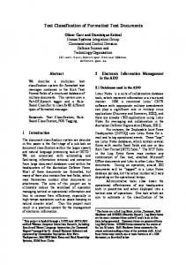
Therefore we use a back-propagation neuronal network with one hidden layer and 16 units in the input layer. For the output layer, to simplify the problem, we decided to use a number of 16 neurons, activating only one neuron at a given moment, according to the predicted class. The best result presented in our previous work, was obtained by the meta-classifier based on cosine, where classification accuracy reached 93.87% on the testing set [5]. The testing set is the same set that is presented in section 5. Fig. IV.1 The architecture of the adaptive meta-classifier M-BP for the training set we also have created a set with the correct answers for each document, based on ratings provided by Reuters [15]. Thus, a response contains the value "1" for the correct class and the value "0" otherwise. The structure of the adaptive metaclassifier based on Back-propagation method (noted M-BP) is shown in Fig. IV.1 5. EXPERIMENTAL FRAMEWORK The Dataset Our experiments are performed on the Reuters-2000 collection [15], which has 984MBytes of newspapers articles in a compressed format. Collection includes a total of 806,791 documents, with news stories published by Reuters Press covering the period from 20.07.1996 through 19.07.1997. The articles have 9822391 paragraphs and contain 11522874 sentences and 310033 distinct root words. Documents are pre-classified according to 3 categories: by the Region (366 regions) the article refers to, by Industry Codes (870 industry codes) and by Topics proposed by Reuters (126 topics, 23 of them contain no articles). Due to the huge dimensionality of the database we will present here results obtained using a subset of data. We selected only the documents for which the industry code value is equal to “System software”, chosen randomly from all 870 industry codes. We obtained 7083 files that are represented using 19038 features and 68 topics. We represent a document as a vector of words; applying a stop-word filter (from a standard set of 510 stop-words) and extracting the word stem [2]. From these 68 topics we have eliminated those topics that are poorly or excessively represented. Thus we eliminated those topics that contain less than 1% documents from all 7083 documents in the entire set. We also eliminated topics that contain more than 99% samples from the entire set, as being excessively represented. After doing this we obtained 16 different topics and 7053 documents, that were split randomly in training set (4702 samples) and testing set (2351 samples). Because of this huge amount of used data in the presented experiments we use only these two sets, without using a cross-validation method. In the feature extraction part we take into consideration both the article and the title of the article. 6. EXPERIMENTAL RESULTS In this section we will present experimental results obtained using different architectures for the neural network included into the adaptive meta-classifier presented in figure IV.1. For training the neural network we used the training set with 4702 documents and for testing the network we used the testing set with 2351 documents. Both sets were first processed using the method presented in Section IV.A (the transposition method) and thus we obtained for each document a vector representation with 16 items.
For the number of neurons from the hidden layer we made a series of experiments starting initially with a small number (17 neurons) and we increased this number in small steps (for example we used 19 neurons, 20 neurons, 32 neurons, 36 neurons, 38 neurons, 52 neurons). In those cases we noticed that at some points the error began to fall very slow because it has begun to fluctuate around that value (the problem become to difficult to be represented by current network architecture). We observed that the network fluctuation occurs at smaller error values when we increase the number of neurons from the hidden layer. We observed also that, sometimes, with increasing the number of neurons in the hidden layer the training time, paradoxically, does not increase (although the number of calculations to be made increases). This fact can be explained because when the number of neurons from the hidden layer increases, for the network becomes easier to represent the problem and therefore it faster converges. Therefore the following results are only for the network architecture with a number of neurons in the hidden layer greater than 96. In [4] are presented also results for a smaller number of neurons on the hidden layers. As a method of assessing the network to avoid over-learning, we decided to suspend the network training when it reaches a certain value of the error (computed using the training set), testing it at that error threshold (using the test set), and continuing the training phase until the next error threshold is reached. Therefore the figures presented will show the progress made by the network, during the learning, on the test set. The error values, in the training phase, are calculated as the sum of all errors obtained for each example belonging to the training set. Since the training set contains 4702 vectors and the error in each vector is a sum of 16 elements, for a long training time the total error will be a value over 1. We will start testing from a total error value equal to 500, representing an average error of 0.11 per sample. The minimum total error value that was reached in experiments is equal to 50 which mean an average error of 0.01 per sample. The evaluation of the network, during the testing phase, will generate the number of incorrectly classified documents, based on the test set. Regarding the rate of learning, it starts with a value equal to 1 for a total error value greater than 350 and decrease in time reaching a value of 0.01 when the total error value became 50. When the network began to fluctuate around a current value of total error we have decreased the learning rate. The experiments presented have started from a number of 96 neurons in the hidden layer. When the time required to reduce the total error between two successive stops become higher (the order of 2-3 hours) we stopped the training for that network configuration. For this reason in the table and figures below some configurations did not reached the minimum error value obtained for the best configuration tested. This is observed as blank spaces in the table presented below.
As methodology for choosing the number of neurons for the hidden layer we used values equal to multiples of 16 and we stopped at a number of 192 neurons on the hidden layer because we believe the results are convincing.
Learning step
Total training error
1 1 1 1 0,9 0,9 0,8 0,8 0,7 0,7 0,6 0,6 0,6 0,6 0,5 0,5 0,5 0,4 0,4 0,3 0,3 0,2 0,2 0,1 0,1 0,1 0,1 0,1 0,1 0,01 0,01 0,01 0,01 0,01
500 450 400 350 340 330 320 310 300 290 280 270 260 250 240 230 220 210 200 190 180 170 160 150 140 130 120 110 100 90 80 70 60 50
In the table VI.1 we present the number of incorrectly classified documents obtained by the designed architectures at the testing points. For each architectural instance we presented the value obtained for all tests performed during the network training process (columns 3-7). Thus the second column presents the total error values when the network training was stopped and tested. The first column presents the corresponding value for the learning step that was used. With bold are represented the maximum values obtained in those stopping points. The figure VI.1 presents the results in terms of classification accuracy for 5 configurations of the neural network architecture. The configuration with 176 neurons in the hidden layer classifies correctly most of the documents in most of the cases. However, this configuration has failed within a reasonable time to decrease the total error below the 80. The best results, if the total training error fell below 100, were obtained by the architecture with 192 neurons in the hidden layer. In this case we obtained only 6 documents incorrectly classified which represent a classification accuracy of 99.74%, while the configuration with only 176 neurons reached a classification accuracy of 99.27%. The figure VI.2 represents the response time for each of the neural network configuration to reach the average errors presented in table VI.1. We mention that the required time for the different configurations to reach the first average error settled, is longer because the network starts using random weights. These weights usually generates a greater value of the average error and the network needs therefore more time to reach the first given error value. At the same time we can observe that time is not continuously increasing with the error decreasing because, in order to reach a certain global error, the network needed sometimes more steps but the general tendency is rising. The implemented metaclassifier runs on a Dual Core Pentium IV at 2.6GHz, with 2GB DDRAM, 300GB HDD at 7200 rpm and Windows VISTA. In [12] the authors present a methodology which calculates the upper limit for the meta-classifier that could be reached based on the number and types of classifiers selected to be contained in the
128
160
176
192
381 345 278 221 214 199 196 186 173 161 155 149 139 123 116 112 108 102 100 91 88 77 76 67 56
369 325 282 226 220 212 209 199 190 177 168 158 147 141 132 124 114 109 104 97 83 80 70 61 57 53 49
368 334 268 223 213 200 194 185 170 170 161 154 146 134 127 120 106 98 87 81 71 68 62 56 46 42 36 32
376 324 282 232 222 206 199 194 184 170 164 154 142 130 124 111 103 91 82 73 64 58 56 43 35 33 27 25 22 21 17
374 321 288 224 217 217 205 195 184 167 160 152 145 132 128 115 99 96 85 76 64 57 53 49 41 35 30 28 23 19 14 12 9 6
non-adaptive meta-classifier. This methodology is based on the number of documents from the testing set that all classifiers, taken 400
96 neurons
350
128 neurons 300 Error thresholds
Classification Accuracy
96
Table VI.1 Number of incorrect classified documents
Influence of the neurons number from the hidden layer 100 99 98 97 96 95 94 93 92 91 90
Number of neurons for the hidden layer
96 neurons 128 neurons 160 neurons
160 neurons
250
176 neurons
200
192 neurons
150 100
176 neurons
50
192 neurons
0
350 320 290 260 230 200 170 140 110 80 Averge error using the training set
Fig. VI.1 Classification accuracy
50
0
10000
20000
30000
40000
Time in seconds
Fig. VI.2 Time necessary for reaching the given total error
separately, fail to correctly classify it. We called these documents "problem documents". The limit obtained in this way was 98.63% and was considered being the maximum limit that can be obtained. This maximum limit depends on the choused dataset and on the used classifiers. By introducing a neural network into the metaclassifier we transformed it into a more adaptive meta-classifier and have shown that the accuracy of 98.63% is not actually a maximum of meta-classification as we previously considered it. As we already prove, due to the supervised adaptive learning, this limit may be exceeded. For example if the maximum element of an input vector is not ranked the right class, it may turn out that it can trigger the activation of the correct unit just because of the properly learning process. CONCLUSIONS AND FURTHER WORK In this article we have developed a meta-classifier based on a backpropagation neural network. This new adaptive meta-classifier uses 8 types of SVM classifiers and one Naïve Bayes type classifier to achieve the transposition of the input data from a large-scale space (in our case 1309 attributes) into a much smaller size space (only 16 attributes), which is suitable for a neural network. The trust degree provided by the transposition method is based on two factors. The first is that it is used as input a large scale representation of the documents (1309 attributes) with benefits to differentiate documents. The second factor is that each classifier returns a vector, where each value represents the confidence given to the current document to be classified in that class. By this transposition we can represent the input data into a space with only 16 dimensions.
We tested and presented in this paper 5 configurations for feedforward neural network architectures that differs by the number of neurons from the hidden layer. The best results (99.74% in terms of classification accuracy) were obtained using a neural network with 192 neurons in the hidden layer. However, comparing the numbers of incorrect classified documents obtained during the testing points, the network with 176 hidden layer neurons was the best one. According to our presented results the developed neural metaclassifier significantly outperforms the previously developed nonadaptive meta-classifiers. Thus, the neural meta-classifier is able to classify the documents that others non-adaptive meta-classifiers failed to "learn". This adaptation was surprisingly successful even if the network was trained on a training set and tested on different testing set. Documents considered "problem documents" are found only in the test set. This new adaptive meta-classifier managed to exceed the maximum "theoretical" limit of 98.63% which could be reached by an ideal non-adaptive meta-classifier that always chose the correct prediction if at least one classifier provide it [3, 13]. As further developments we will try to improve the implementation of the neural network so it will more quickly converge. Also it is interesting to test other transposing methods that would generate the results more quickly and more accurate, too. [1]
REFERENCES P. Bennett, Building Reliable Metaclassifiers for Text Learning, PhD Thesis - School of Computer Science, Carnegie Mellon University Pittsburgh, http://reportsarchive.adm.cs.cmu.edu/anon/2006/CMU-CS-06-121.pdf, 2006.
[2] [3]
[4] [5] [6]
[7] [8]
[9]
[10]
[11] [12]
[13] [14] [15] [16] [17] [18]
S. Chakrabarti, Mining the Web- Discovering Knowledge from hypertext data, Morgan Kaufmann Press, 2003. R. Cretulescu, D. Morariu, L. Vinţan, Eurovision-like weighted Non-Adaptive Metaclassifier for Text Documents, The 8th RoEduNet International Conference, Galaţi, Romania, December 2009. R. Cretulescu, Meta-classifier based on Neural Network, 3rd PhD Report, “Lucian Blaga” University of Sibiu, 2009, http://webspace.ulbsibiu.ro/radu.kretzulescu/html/phdreport3.pdf. R. Cretulescu Support Vector Machine versus Bayes Naïve, 2nd PhD Report, “Lucian Blaga” University of Sibiu, 2008, http://webspace.ulbsibiu.ro/radu.kretzulescu/html/phdreport2.pdf. N. Dimitrova, L. Agnihotri and G. Wei, Video Classification Based on HMM Using Text and Face, Proceedings of the European Conference on Signal Processing, Finland, 2000. D. Lewis, Naive (Bayes) at Forty: The Independence Assumption in Information Retrieval, In Proceedings of the 10th European Conference on Machine Learning, 1998. W.-H. Lin, A. Hauptmann, News Video Classification Using SVM-based Multimodal Classifier and Combination Strategies, In Proceedings of the Tenth ACM international Conference on Multimedia, 2002. W.-H. Lin, R. Jin, A. Hauptmann, A Meta-classification of Multimedia Classifiers, International Workshop on Knowledge Discovery in Multimedia and Complex Data, 2002. C. Hua Li, S. Cheol Park, A Novel Algorithm for Text Categorization Using Improved Back-Propagation Neural Network, Proceedings of the 3rd International Conference Fuzzy Systems and Knowledge Discovery , Xi’an, China, September 2006. H. Jaiwei, Micheline K., Data Mining. Concepts and techniques, Morgan Kaufmann Press, 2001. D. Morariu, L. Vinţan, V. Tresp, Meta-Classification using SVM Classifiers for Text Documents, The 3rd International Conference on Neural Computing and Patter Recognition, Barcelona, October 2006. D. Morariu, Text Mining Methods based on Support Vector Machine, MatrixRom, Bucharest, 2008. C. Nello, J. Swawe-Taylor, An introduction to Support Vector Machines, Cambridge University Press, 2000. Reuters Corpus: http://about.reuters.com/researchandstandards/corpus/ Released in November 2000. B. Schoelkopf, A. Smola, Learning with Kernels. Support Vector Machines, MIT Press, London, 2002. G. Siyang, L. Quingrui, M. Lin, Meta-classifier in Text Classification, http://www.comp.nus.edu.sg/~zhouyong/papers/cs5228project.pdf. N. L. Vinţan, Prediction Techniques in Advanced Computing Architectures, Matrix Rom, Bucureşti, 2007.