An Adaptive Multimodal Biometric Management Algorithm - Kalyan ...

344

IEEE TRANSACTIONS ON SYSTEMS, MAN, AND CYBERNETICS—PART C: APPLICATIONS AND REVIEWS, VOL. 35, NO. 3, AUGUST 2005

An Adaptive Multimodal Biometric Management Algorithm Kalyan Veeramachaneni, Lisa Ann Osadciw, Senior Member, IEEE, and Pramod K. Varshney, Fellow, IEEE

Abstract—This paper presents an evolutionary approach to the sensor management of a biometric security system that improves robustness. Multiple biometrics are fused at the decision level to support a system that can meet more challenging and varying accuracy requirements as well as address user needs such as ease of use and universality better than a single biometric system or static multimodal biometric system. The decision fusion rules are adapted to meet the varying system needs by particle swarm optimization, which is an evolutionary algorithm. This paper focuses on the details of this new sensor management algorithm and demonstrates its effectiveness. The evolutionary nature of adaptive, multimodal biometric management (AMBM) allows it to react in pseudoreal time to changing security needs as well as user needs. Error weights are modified to reflect the security and user needs of the system. The AMBM algorithm selects the fusion rule and sensor operating points to optimize system performance in terms of accuracy. Index Terms—Multisensor fusion, multimodal biometrics, particle swarm optimization.

I. INTRODUCTION IOMETRICS is an attempt to imitate the elegant sensor fusion network of humans in identifying and verifying other humans by their behavioral and physiological characteristics” (a self quote from Lisa Kalyan). The first modern commercial biometric device was introduced over 25 years ago when a machine that measured finger length was installed for maintaining employee time records at Shearson Hamil on Wall Street. In the ensuing years, hundreds of these hand geometry devices have been installed for security purposes at facilities operated by Western Electric and Naval Intelligence. In the US today, biometric security systems may be found in the Oakland International Airport (face recognition), Chicago O’Hare International (fingerprint), and the Navy Consolidated Building (iris recognition) [1]. With an increasing demand for better security technology in public and private buildings since September 11, 2001, a variety of pilot projects have been completed in the area of access control [2]. These projects highlight the need to improve biometric verification accuracy, universality, and ease of use. Identification methods can be grouped into three classes: something you possess as in an ID card, something you know, and something unique about you. Possessions (e.g., keys) can be easily lost, forged, or duplicated. Knowledge can be forgotten as well as shared, stolen, or guessed. The cost of forgotten passwords is high and accounts for 40%–80% of all the IT help

“B

Manuscript received March 15, 2003; revised December 20, 2003. This paper was recommended by Guest Editor D. Zhang. The authors are with the Department of Electrical Engineering and Computer Science, Syracuse University, Syracuse, NY 13244 USA. Digital Object Identifier 10.1109/TSMCC.2005.848191

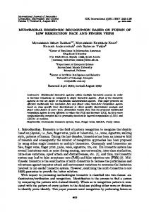
desk calls [3]. Resetting the forgotten or compromised passwords costs as much as $340/user/year [4]. Biometrics, which is something unique about you, are inherently secure since they are unique features the person has. The science of biometrics is a solution to identifying an individual and avoids the problems faced by possession-based and knowledge-based security approaches. The aggregate security level of a system increases as these three identification approaches are combined in various ways. The least secure approach is one based solely on Personal Identification Numbers (PINs). This is because a very small PIN consisting of four characters can be easily guessed by an imposter, while a 200-character PIN is difficult for users to remember. This often leads to PINs getting compromised in many ways, such as a second possession. The biometrics system’s security level can be improved by adding some possession such as an identification card. Finally, additional possessions with multiple biometrics support a very high security level, as illustrated in Fig. 1. This paper proposes an approach supporting highly secure systems that utilize multisensor fusion to improve the security level of a system by combining biometric modalities. An algorithm is presented that adaptively derives the optimum Bayesian fusion rule as well as individual sensor operating points in a system. The algorithm bases its design on system requirements, which may be time-varying. Other researchers have published numerous experimental results demonstrating the effectiveness of fusion in biometrics [5]–[10]. Ad hoc techniques have been demonstrated to be effective but not always optimum in terms of accuracy [9], [10]. For example, the BioID system [9] chooses from different fusion strategies to vary the system security levels. The fusion options, however, contain only a few fusion rules, typically the “and” and “or” rules, severely restricting the rule search. The decision thresholds or operating points for individual sensors are fixed in these systems, which fixes the false acceptance rate (FAR ) and false rejection rate (FRR ). This approach successfully reduces FAR or FRR [10] but not both. In contrast, the adaptive, multimodal biometric management algorithm (AMBM), which is presented in this paper, comprehensively considers all fusion rules and all possible operating points of the individual sensors. The optimum Bayesian fusion rule is designed based on the current situation as it is defined by the Bayesian error costs. As the situation changes with time, AMBM revises the fusion rule and the sensor operating points. This paper describes this novel sensor management algorithm and how it is applied to the biometric security application. The block diagram shown in Fig. 2 presents the AMBM algorithm in detail. The system has N biometric sensors, a Particle Swarm Optimizer (PSO), a Bayesian Decision Fusion processor, and a Mission manager. The mission manager provides the PSO the

1094-6977/$20.00 © 2005 IEEE Authorized licensed use limited to: Syracuse University Library. Downloaded on June 23, 2009 at 08:57 from IEEE Xplore. Restrictions apply.

VEERAMACHANENI et al.: AN ADAPTIVE MULTIMODAL BIOMETRIC MANAGEMENT ALGORITHM

Fig. 1.

Approaches to increasing security needs.

Fig. 2.

Illustration of adaptive multimodal biometric fusion algorithm.

costs, which reflect system requirements. The PSO searches for an optimal configuration of the sensors with a corresponding fusion rule matching those requirements. The threshold values for each biometric sensor are also selected since they are function of the sensor FAR determined by the PSO. These sensors now operate at these thresholds determined by the PSO. The Bayesian Decision Fusion processor fuses the decisions from multiple sensors using the optimum fusion rule from the PSO into a final decision. New rules and thresholds are found when the PSO receives new costs from the mission manager. The next section provides a quick review of the existing biometric technologies discussed in this paper. The third section describes how the Bayesian decision fusion framework sup-

345

ports automated adaptivity. The fourth section presents the new AMBM algorithm with its evolutionary algorithm PSO. The final section summarizes the results and presents conclusions. II. REVIEW OF EXISTING BIOMETRIC TECHNOLOGIES The paper focuses on three modalities: face recognition, voice recognition, and hand geometry comparisons. The three biometric sensors referenced in this paper are a face recognition system by Visionics, a hand biometric system by Recognition Systems, and a voice recognition system by OTG using the SecurPBX demonstration system [11]. The experimental data referred to in the third section of the paper focussed on the three biometric sensors and was collected and analyzed by

Authorized licensed use limited to: Syracuse University Library. Downloaded on June 23, 2009 at 08:57 from IEEE Xplore. Restrictions apply.

346


TABLE I USER TRANSACTION TIMES IN SECONDS

face images (training faces) in the database. Face recognition accuracy suffers from the inherent variations in the image acquisition process in terms of image quality, geometry, illumination effects, as well as occlusions (glasses, facial hair, etc.). These major problems currently limit the accuracy of face recognition. C. Voice Verification

Mansfield et al. A volunteer crew of 200 employees was used to test the biometric devices. A detailed approach about the methodology of determining the receiver operating curves (ROCs) for the above three sensors is given in [11]. These particular sensors differ in their universality, ability to extract unique features from the entire user population, and ease of use. The sensors are comparable in accuracy; this prevents a single modality from severely dominating the fusion process. The fusion management algorithm, however, can be applied to any set of biometric sensors with very simple modifications. Transaction time or the time required to collect biometric data is another performance parameter that led to the selection of the three modalities currently considered. The transaction times in Table I (in seconds) were experimentally determined for various biometric modalities in [11]. The transaction times include multiple attempts allowed for each user [11] and, hence, are longer than usual. The study by Mansfield et al. [11] stated that users are sensitive to transaction times exceeding 30 s. In order to maintain user-acceptable transaction times, the modalities in this paper have been chosen so that the system can collect multiple features within 30 s. This requires the features to be collected simultaneously. For example, face and voice features have the longest transaction times but the mean transaction time can be reduced from 37 to 22 s if the data are simultaneously collected. Each biometric technology must perform four basic tasks: biometric acquisition, feature extraction, matching, and decision making, as shown in Fig. 2. AMBM fuses the single sensor decisions. The next three subsections briefly describe the various biometric technologies referenced in this paper. A. Hand Geometry Comparisons Hand geometry is extremely user-friendly but has lower accuracy when compared to fingerprinting and iris scanning [12]. The lengths of the fingers as well as other hand-shape attributes are extracted from images and used in a feature representation of the hand. A relatively inexpensive camera can be used to acquire the features resulting in a low-cost system. Hand geometry systems, however, have relatively high FAR and FRR values. In a hand recognition system, jewelry such as rings can cause errors. Hand injuries also adversely affect the system accuracy. B. Face Recognition Human beings have always used face recognition for personal identification purposes. In automatic face recognition, computer systems use feature sets to match the test face image (newly acquired and unknown) against a single or collection of known

Voice verification, like face recognition, is attractive because of its prevalence in human communication. Speaker identification suffers considerably from variations in the microphone and/or the transmission channel. The performance deteriorates badly as enrollment and acquisition conditions become increasingly mismatched. Background noise is a considerable problem. Variations in voice due to illness, emotion, or aging are other problems requiring further research. III. MULTIMODAL FUSION WITH AN ADAPTIVE BAYESIAN DECISION FRAMEWORK Recently, there has been a lot of interest in multimodal biometric identification systems [7], [8]. As discussed in the previous section, each modality has its own limitations, issues, and problems. One approach to improving biometric identification accuracy is solving the problems facing each biometric technology. This does not, however, address the issue of universality. The only approach to identifying someone who cannot provide a unique feature for a particular biometric modality is to use multiple modalities. For example, fingerprinting will never work for someone without hands. The approach described in this paper can address all the issues facing a biometric security system through adaptable integration of multiple sensors. Multimodal biometric fusion systems can be broadly categorized based on the type of information extracted from the sensor. In Fig. 3, these fusion categories are feature-level fusion, scorelevel fusion, and decision-level fusion [7]. Decision-level fusion is the most abstract level and consolidates multiple accept/reject decisions from multiple sensors into one decision. This approach takes advantage of the tailored processing performed by each biometric sensor. It also requires the least communication bandwidth and, thus, supports scalability in terms of the number and types of biometric sensors. Feature and score level fusion, however, have been shown to enhance accuracy to a greater degree than decision-level fusion. As the sensors become more dissimilar, however, feature- and score-level fusion become more complex, if not impossible, to accomplish. The next subsection describes the Bayesian decision fusion framework used in AMBM. A. Accuracy in the Bayesian Framework A Bayesian framework can be used as the basis of a fusion system that automatically adapts the security level as well as reacts to changes in the user’s physical characteristics [12]. As a brief review, the problem of personal identification can be formulated as a hypothesis testing problem where the two hypotheses are as follows. H0 The person is an imposter.



Fig. 3.

347

Levels of fusion.

H1 The person is genuine. The conditional probability density functions are p(ui |H1 ) and p(ui |H0 ), where ui is the decision of the ith biometric sensor given the genuine person and the imposter, respectively. The decision made by sensor i is 0, person is an imposter (1) ui = 1, person is genuine The Bayesian cost, which is the error measure focused on in this paper, is based on the inaccuracy of the fusion system. It is composed of two types of error rates: the false rejection error rate and the false acceptance error rate. The false acceptance rate is the conditional probability of declaring someone as genuine if he is actually an imposter or FARi = P (ui = 1|H0 ).

(2)

The false rejection rate is the conditional probability of declaring someone an imposter if he is actually genuine or FRRi = P (ui = 0|H1 ).

(3)

Since the algorithm is in a Bayesian framework, a Bayesian cost for the system is obtained from a weighted sum of the two global errors FAR and FRR . The global errors are computed based on the fusion rule and the individual sensor errors: (2) and (3). The computation of the global errors is discussed in more detail in Section IV. The Bayesian cost, minimized by the appropriate fusion rule, is E = CFA FAR + CFR FRR

(4)

where CFA is the cost of falsely accepting an imposter, CFR is the cost of falsely rejecting the genuine individual, FAR is the global false acceptance rate, and FRR is the global false rejection rate. This can be rewritten in terms of a single cost using CFR = 2 − CFA

(5)

E = CFA FAR + (2 − CFA )FRR .

(6)

giving

Equation (5) results from the fact that the global error is historically simply the sum of the two error rates if cost is ignored. Thus, the costs are assumed to be 1. The optimum Bayesian fusion rule minimizes the Bayesian cost (6) by selecting the rule and all single sensor operating points. The single sensor

Fig. 4.

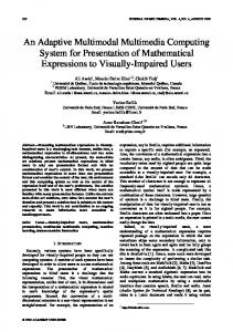
Experimentally determined operating curves for 3 biometrics.

observations and the corresponding decisions are assumed to be independent. The performance of a biometric sensor is often represented in terms of ROCs or a plot of genuine acceptance rate (GARi ) versus FARi . The genuine acceptance rate for sensor i is GARi = 1 − FRRi .

(7)

Fig. 4 contains the ROC curves experimentally determined for the three sensors previously discussed [11]. An ROC for the fused systems can also be found for each Bayesian fusion rule using the FAR and the fused system’s GAR where GAR = 1 − FRR .

(8)

Fig. 5 plots ROCs for the AND and OR rules applied to face and voice recognition systems. The AMBM algorithm finds the optimum decision rule that minimizes the system’s Bayesian cost (6). The AMBM algorithm uses the given error costs and searches through the space of all possible rules and the sensor operating points. The sensor operating point is defined by a decision threshold that determines a sensor’s FARi and FRRi . Gaussian noise is assumed for the probability density functions (pdf) conditioned on the decision hypotheses. This assumption is supported by


348


Fig. 7.

Fig. 5.

Thresholding in terms of pdfs versus scores for sensor 2 (first example).

ROC for two sensors.

Fig. 8. Thresholding in terms of pdfs versus scores for sensor 1 (second example). Fig. 6.

Thresholding in terms of pdfs versus scores for sensor 1 (first example).

the experimental data collected by Mansfield et al. Simulated pdfs based on experimental pdfs are used to model sensor performance and plotted in Figs. 6–9. These models are a close approximation of the experimental data in [11]. These models are key to AMBM using an evolutionary search technique to find the optimum decision fusion rules. The models can be modified in pseudoreal time to reflect changes in a sensor’s performance, degradation, or improvement. If the security must be heightened or reduced, the system can react in real time, modifying the cost of false acceptance. A new optimum rule will be selected in response to a change in the error costs or sensor performance. B. Optimum Bayesian Decision Framework A Bayesian framework can be automatically adapted by selecting the FAR cost and FRR costs to reflect the security level and uniqueness of the user’s biometrics. The decision concern-

Fig. 9. Thresholding in terms of pdfs versus scores for sensor 2 (second example).



TABLE II FUSION RULES FOR TWO SENSORS

ing a person’s genuineness is made through the following likelihood ratio test p(ui |H1 ) ui =1 >< λi p(ui |H0 ) ui =0

349

(9)

where λi is an appropriate threshold [13]–[15]. Four possible decisions are as follows. 1) The genuine person is accepted. 2) The genuine person is rejected. 3) The imposter is accepted. 4) The imposter is rejected. The optimum Bayesian fusion rule allowing access to a building for N sensors is [14], [15] 1 − FRRi FRRi ui log + (1 − ui ) log FARi (1 − FARi ) i=1 ug =1 CFA >< log (10) 2 − CFA ug =0

N

where ug is the global decision, and ui is the decision of the ith sensor. The rule in (10) assumes an equal a priori probability of an imposter and genuine user. This assumption is based on the system’s lack of knowledge concerning this factor. This parameter may be added to (10) if the probabilities are known N and not equal. There is a total of 22 possible fusion rules for N sensors.

rule allows everyone in. The system can completely ignore one sensor by using the f4 (sensor 1) or f6 (sensor 2) rules. In order to gain insight into the performance enhancements resulting from the fusion of two sensors, we present the global FAR and FRR as functions of the individual sensor FARi and FRRi for two rules: AND and OR rules. The two-sensor FAR and FRR for the AND rule are (11)

FRR = FRR1 + FRR2 − FRR1 FRR2 .

(12)

and

C. Effects of Cost on Rule Selection By changing the Bayesian costs and directly modifying the optimum fusion rule in (10), the system can automatically vary its performance, which is defined by (4). The system performance is tightly tied to system accuracy in this paper. This is entirely a result of the system’s purpose: security. It is a straightforward modification to AMBM to incorporate additional performance factors. These factors, however, do not affect the optimum Bayesian fusion rule in (10). If security is heightened, this system increases the cost of false acceptance. AMBM then finds the rule and sensor operating points to meet a cost that is driven by the Bayesian cost. For example, if everyone temporarily requires access to the building, the cost of admitting an imposter (CFA = 0) may be set at 0. Conversely, the cost for falsely rejecting a genuine user becomes 2. For this situation, the optimum rule is simply 1 for every access attempt, allowing everyone access. For the fusion of the face and voice biometric sensor decisions, there are 16 potential rules possible, as depicted in Table II. The rules are represented by binary strings since the decisions are binary (i.e., imposter or genuine user). The optimum fusion rule of 1 is f16 , for example. It has been proven that an optimum fusion rule for any set of Bayesian costs is monotonic in [15], so all other rules can be ignored by AMBM. The most commonly used rules are f2 (AND rule) and f8 (OR rule). The NAND rule or f9 is rarely of interest since it typically performs poorly. The f1 rule simply allows no one in the building and can be used to lock up a building. Similarly, the f16

FAR = FAR1 FAR2

It is apparent that this improves FAR while degrading the FRR . The GAR decreases as well. The degradation can be significant if the two sensors are not comparable in terms of accuracy. The OR rule reverses this effect giving FAR = FAR1 + FAR2 − FAR1 FAR2

(13)

FRR = FRR1 FRR2 .

(14)

and

The ROCs for these two rules (see Fig. 5), support a comparison of the rules’ performance. The OR rule ROC quickly falls off as the FAR decreases. Thus, the OR rule does not achieve as high a GAR for low FAR values. There is a point between FAR values 0.001% and 1%, where the two curves cross. This crossover point is related to single sensor accuracy. For larger FAR values, the OR rule works to improve performance in terms of GAR . For lower FAR values, the AND rule improves GAR . This example demonstrates that for two sensors, the performance gain is constrained by the less-accurate sensor. One must select to improve either the FAR or FRR but not both. Both error types may be reduced with the addition of a third biometric sensor with better accuracy characteristics than the first two sensors. The problem of analyzing all possible rules, however, begins to become more complex as there are now 3 potentially 22 or 256 fusion rules. Once again, most of these rules can be ignored due to the monotonic constraint, leaving only 20 rules [15]. For added insight, a comparison in Fig. 10 is


350


TABLE III OPTIMAL FUSION RULES FOR SAME OPERATING POINT (FAR1 = FAR2 = FRR1 = FRR2 = 10%)

TABLE IV OPTIMAL SENSOR RULES IF ONE SENSOR DOMINATES FRR (FAR1 = 9%, FRR1 = 0.6%, FAR2 = 1%, FRR2 = 4%)

Fig. 10.

ROC comparison for AND rule.

made between hand, face, and voice verification sensor systems in terms of the ROC’s assumption that the AND rule is used. The ROC shifts from the lower right for one sensor to the upper left for three sensors, demonstrating global accuracy improvement for most FAR values as more sensors are added. The three sensor system provides a higher GAR for the same FAR value. However, the single voice biometric performs better than the two and three sensor systems for very high FAR values. Another fusion rule is optimal and performs better for this range of FAR values. The AMBM algorithm can vary FAR cost in (4) to increase the impact of either error type. The local decisions are first weighted by the accuracy of the sensors’ current operating points and then compared with a threshold in (10). If the costs are equal, the threshold on right side of (9) is 0. The threshold increases as the cost of FAR increases. The rule accounts for the inherent accuracy of the sensor through the single sensor accuracy values on the left side of (9). The sensor decisions are incorporated through ui on the left side of (9) as well. For example, a table of optimal fusion rules as a function of FAR costs can be constructed as shown in Table III. Identical sensors with the same operating point were used to generate the table. This would also correspond to the use of multiple attempts to attain access using the same biometric sensor if independence is assumed. If the FAR is more costly (CFA = 1 to 1.976), the AND rule is optimal. If the FRR is more costly (CFA = 0.0024 to 1), the OR rule is optimal. There is a very small range of costs (CFA = 0 to 0.0024) that allows everyone access. Another small cost range (CFA = 1.976 to 2) corresponds to rejecting everyone’s access. The OR and AND rules transition at a cost equal to 1 (i.e., when both errors are equally costly).

In contrast, another set of sensor operating points, where one sensor dominates in either FAR or FRR , is summarized in Table IV. In this example, sensor 1 dominates FRR but has a poor FAR . Sensor 2 has better FAR values. The AMBM algorithm must use Sensor 2’s FAR to improve the global FAR by using the AND rule. The table indicates that the AND rule remains optimal for FAR costs ranging from 1.9982 through 0.7752. Conversely, the OR rule becomes optimal for FAR costs of 0.6172 to 0.000 532 6. It is important to note that the optimum fusion rule for FAR costs between 0.6172 and 0.7752 relies on only one sensor, sensor 2. Fig. 11 plots the Bayesian cost as a function of FAR cost for the three primary rules selected in Table IV. The lines cross at the points where the optimum rule switches. The costs and rules change for every set of sensor operating points selected. The next section describes the AMBM algorithm that uses cost, operating points, and fusion rules to adapt the system’s global accuracy. IV. ADAPTIVE MULTIMODAL BIOMETRIC MANAGEMENT ALGORITHM The AMBM algorithm, as introduced previously, is composed of three major components: a particle swarm optimizer (PSO), a mission manager, and the Bayesian fusion processor (Fig. 2). The PSO, which is key to the success of AMBM, has been designed to search the global fusion rule space, which is binary, and the sensor operating point space, which is continuous. The optimum rule is selected and passed to the fusion processor. Finally, the Bayesian fusion processor applies the optimum rule to make global decisions from the local decisions as users access



351

TABLE V FUSION RULE FORMATION FOR TWO SENSORS

global best position Pg . The velocity is updated by [18]–[20] (t+1) (t) (t) Vmd = ω × Vmd + rand(1) × Ψ1 × pmd − Xmd (t) (15) + rand(1) × Ψ2 × pgd − Xmd and the position is updated by Fig. 11.

(t+1)

Cost versus PSO total cost for the operating point in Table IV.

the system. The costs of the system errors, which are computed in the mission manager, are dependent on many factors. This section focuses on the unique PSO used in AMBM. A. PSO Approach PSO was originally introduced in terms of social and cognitive behavior by Kennedy and Eberhart in 1995 [16]. PSO has come to be widely used as a problem-solving approach in engineering and computer science and has since proven to be a powerful competitor to genetic algorithms [17]. This approach is simple and comprehensible as it is derived from the social behavior of individuals such as birds, fish, and other subjects of swarming theory. The individuals, called particles, are flown through the multidimensional search space. Each particle tests a possible solution to the multidimensional problem as it moves through the problem space. The movement of the particles is influenced by two factors: the particle’s best solution (pbest) and the global best solution found by all the particles (gbest). These factors influence the particle’s velocity through the search space by creating an attractive force. As a result, the particle interacts with all the neighbors and stores in its memory optimal location information. After each iteration, the pbest and gbest are updated if a more optimal solution is found by the particle or population, respectively. This process is continued iteratively until either the desired result is achieved or the computational power is exhausted. The PSO formulas define each particle in the D-dimensional space as Xm = (xm1 , xm2 , xm3 , . . . xmD ), where the subscript m represents the particle number, and the second subscript is the dimension. The memory of the previous best position is represented as Pm = (pm1 , pm2 , pm3 . . . pmD ) and a velocity along each dimension as Vm = (vm1 , vm2 , vm3 . . . vmD ) [18]. After each iteration, the velocity term is updated. The particle’s motion is influenced by its own best position Pm , as well as the

Xmd

(t)

(t+1)

= Xmd + Vmd

.

(16)

Constants Ψ1 and Ψ2 determine the relative influence of the pbest and gbest. Often these are set to same value giving equal weight to both. The memory of the PSO is controlled by ω. Each particle in this problem has “N + 1” dimensions, where N is the number of sensors in the sensor suite. The first N dimensions are the sensor thresholds for all sensors in the sensor suite. The (N + 1)th dimension is the fusion rule, which determines how all the decisions from the sensors are fused. Hence, the representation of each particle is Xm = {λm1 , λm2 , λm3 , . . . , λmn , fm }.

(17)

The sensor thresholds are continuous. In contrast, the fusion rule (f ) is a binary string having a length of s = log2 p N

(18)

where p = 22 . The rule f may be represented by an integer value varying from 0 ≤ f ≤ p − 1. This proved to be inefficient due to all the bounding that was required in AMBM. For this binary search space, the binary decision model and search strategy as described in [19] are being used. This binary decision model results in a much faster convergence than the integer number model. In the algorithm instead of evolving the thresholds explicitly, the false acceptance rates (FAR ) are evolved in the PSO for each of the sensors. Thresholds are calculated based on the FAR and sensor models determined a priori and updated. The PSO minimizes the cost, (6). The global FAR and the FRR for the optimum fusion rule f are calculated directly from the fusion rule and individual sensor FARi and FRRi . For example, with two sensors, the fusion rule consists of 4 bits, as represented in Table V. In Table V, u1 is the first sensor decision, and u2 is the second sensor decision. The global decision replaces {d0 , d1 , d2 , d3 } with 0s and 1s in their respective locations within f . The global


352


TABLE VI MEANS AND STANDARD DEVIATIONS OF THE GAUSSIAN DISTRIBUTIONS FOR TWO SENSORS

TABLE VII PSO PARAMETERS

TABLE VIII TABLE CONTAINING THE RESULTING OPERATING POINTS AND ERROR RATES AFTER 10 000 ITERATIONS

error rates can then be computed directly from   s−1 N FAR = di ×  ΨARj  i=0

where

ΨARj =

1 − FARj , (uj = 0) (uj = 1) FARj ,

and

s−1 N (1 − di ) ×  ΨRRj  i=0

where

ΨRRj =

(20)





FRR =

(19)

j=1

(21)

j=1

FRRj , (uj = 0) 1 − FRRj , (uj = 1)

(22)

The PSO cost function, which is the objective function optimized by the PSO, is Ea = CFA × (FARa − FARd ) + (2 − CFA ) × (FRRa − FRRd ) .

(23)

FARa and FRRa are the achieved global false acceptance and rejection rates estimated using the a priori sensor models. FARd and FRRd are the desired global false acceptance and rejection rates from the mission manager. AMBM adapts to the required error rates preventing overdesign of the rule by using (20) as the PSO objective function. B. PSO Performance This section demonstrates the effectiveness of the swarm in selecting the optimal rule and operating points dynamically to meet the general security requirements of the system. The results of AMBM for the two false acceptance costs of 1.8 and 1.9 demonstrate the volatility of the algorithm. The same a priori sensor models are used in both runs. Table VI contains the means and standard deviations used in selecting the sensor operating points if Gaussian distributions are assumed. These distributions are important to the PSO because they provide a model that is continuous over the region of operation. This infinite search space requires an evolutionary search approach. The distribution parameters are used by the swarm to compute the threshold and the false rejection rate for any particular false acceptance rate. The sensor operating points are passed to the sensors modifying their individual operation as shown in Fig. 2. The sensor’s new

threshold is applied in the decision processing illustrated in Fig. 3. Thus, the AMBM modifies the single sensor operation through its threshold feedback. Figs. 6–9 show the thresholds in terms of “score” on the x-axis. The swarm parameters used for the run are shown in Table VI. Table VIII shows the results obtained by running the swarm with CFA = 1.9 and CFA = 1.8, respectively. Although the cost has been decreased by only 0.1, the swarm switches from an AND rule to an OR rule with very different operating point sets. For the higher cost of 1.9, the swarm converged to a final solution after 550 iterations. The slightly lower cost of 1.8 took much longer with a solution emerging after 3500 iterations. A balance must be maintained in the choice of the swarm parameters such as ω, which controls memory, to assure convergence as well as prevent premature convergence. A suboptimal solution may be reached if premature convergence occurs, which is the primary risk in using any evolutionary algorithm approach. In this example, the dominance of sensor 2 in terms of accuracy slows convergence of the PSO. The false acceptance costs are set very high, 1.8 and 1.9, so that the optimal solution seems counterintuitive initially and requires careful analysis. For the CFA of 1.8 case, Figs. 6 and 7 illustrate the sensor distributions and thresholds to be used with the OR fusion rule after 10 000 iterations. The threshold for sensor 1 is extremely high, giving a more acceptable false acceptance rate but high genuine user rejection rate (64%); thus, sensor 2 is relied on most of the time. This aligns with the final selection of the OR rule. The PSO cost is 0.0138, indicating that the desired performance criteria is nearly met. The PSO cost plotted as a function of swarm iteration is given in Fig. 12. It is interesting to note that if the AND rule is applied instead of the OR rule as selected by AMBM for these sensor thresholds, the PSO cost increases dramatically to 0.1270. For the second case with CFA = 1.9, the AND rule is selected by the swarm. The details are given in Table VIII after 1000 iterations. The operating point for sensor 2 is nearly identical to the previous case as illustrated in Fig. 9. Sensor 1’s threshold, however, is reduced significantly in Fig. 8. Sensor 1 now has



353

TABLE IX TABLE SHOWING THE RANGES OF CFA AND CORRESPONDING RULE

V. AMBM PERFORMANCE RESULTS

Fig. 12.

PSO cost versus PSO iteration (first example).

Fig. 13.

PSO cost versus PSO iteration (second example).

a higher rate of false acceptance but a more tolerable false rejection rate. The accuracy of sensor 2 is used to offset the high false acceptance rate of sensor 1. The PSO cost is nearly the same as in the previous case (0.0102). If the wrong rule such as the OR rule is applied, the PSO cost increases to 0.9116. Fig. 13 represents the minimum of PSO cost achieved by the swarm after each iteration. This PSO cost plot illustrates the step characteristic, which results from the current minimum PSO cost being maintained until a better PSO cost is found. The swarm particles are moving through the search space testing different parameter sets and sharing their best solutions. When a new global best solution is found, the minimum PSO cost and the particles’ memory are replaced with the newly found better solution. Convergence occurs when all particles produce the same minimum Bayesian cost. It is possible for the particles to present more than one optimal solution in this search space. If multiple solutions yield the same PSO cost, the solutions are viewed as being on the Pareto surface. Any one of the resulting solutions can be selected as a final solution. In such a case, other constraints such as transaction time and ease of use may be introduced to select the most desirable solution.

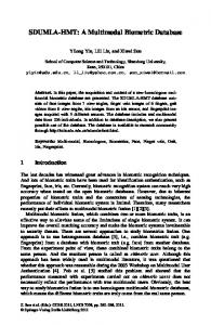
This section presents the solutions lying on the Pareto surface for the complete range of costs (0 through 2). A Monte Carlo simulation ran the AMBM algorithm 100 times for the same cost with 1000 iterations per run. The biometric sensor suite consists of two sensors, which are modeled by the Gaussian distributions described in Table VI. In this case, sensor 2 is more accurate and dominant in the sensor suite. Each Monte Carlo run successfully converged to an appropriate solution with comparable minimum PSO costs for every false acceptance cost. Although the runs did not consistently select the same solution, the selected solution met the AMBM performance criteria. The solutions consist of the rule and the sensor operating point defined by its false acceptance rate and false rejection rate in Table VI. The sensor threshold can be computed from the sensor’s error rates and distributions. Fig. 14 shows the percentage of trials for which a particular rule has been selected as a function of the false acceptance cost. Table IX summarizes the results showing the ranges of costs and the most probable rule selected. The “OR” rule, f8 , is more probable when the cost of false acceptance is low (0–0.5). Due to sensor 2’s dominance, there is a range of costs (0.5–1.5) for which the system simply ignores sensor 1’s decisions. For higher costs of false acceptance (1.5–1.9), the “AND” rule f2 is most frequently selected. The swarm optimization algorithm, however, is able to find multiple solutions involving different fusion rules for one particular global false acceptance cost with equivalent PSO costs. For example, the swarm selected rule f2 76% of the time, f6 19% of the time, and f8 5% for a CFA of 1.9. A comparison of these three rules (for a CFA of 1.9) in terms of minimum PSO cost indicates two things: The operating points were different and standard deviation of the minimum PSO cost was as low as 6.9 e-04 with a mean of 0.0105. The operating points of sensors differed according to the selected rule as demonstrated in Table X. The low standard deviation of the resulting minimum PSO cost (6.9 e-04 for a CFA of 1.9) over the 100 trials indicates that optimality has been achieved independently of the rule chosen. Thus, the AMBM algorithm selected optimal rules and sensor operating points for two sensors with approximately equal PSO costs. A second example is provided in Table X for a cost of 0.1. The operating points and rules are very different for nearly equal PSO costs. This can be extended to any number of sensors in the sensor suite. Table XI shows the values for two more costs, i.e., CFA = 1.4 and CFA = 1.6. AMBM selects f6 40% of the time for a cost of 1.4 and f2 56% of the time for a cost of 1.6. The swarm also selects the operating points to achieve optimal solutions.


354

Fig. 14.


Probability of selecting fusion rule versus cost of false acceptance. TABLE X DETAILED ANALYSIS OF PSO SOLUTION DEMONSTRATING CONVERGENCE

TABLE XI COMPARISON ANALYSIS OF MOST PROBABLE PSO SOLUTION OVER SMALL COST DIFFERENCE

With a cost of 1.4, the swarm uses only a single sensor—sensor 2—which has higher accuracy, and ignores the other sensor. Sensor 1’s operating parameters actually do not matter for this case and have no impact on performance. As the cost of false acceptance increases to 1.6, AMBM selects the AND rule so

that even sensor 1 is needed to achieve the desired accuracy. In conclusion, the analysis of the rules and sensor configurations in Tables IX–XI support the following: the use of false acceptance cost as a mechanism to effectively control system performance and PSO’s ability in finding an optimal solution for different



costs (CFA ) by changing operating points of each sensor as well as the fusion rule. VI. SUMMARY AND CONCLUSIONS The paper presents a novel sensor management algorithm that controls decision fusion and meets the global performance needs of a biometric personal identification system. Cost of false acceptance is a weighting parameter that is used to adaptively control the system’s performance in real time. For example, if the security level is normally operating with a CFA of 1.4, the users are required to provide only a single biometric via sensor 2. This is assuming the same biometric sensor suite that is dominated by sensor 2 in Table VI. If the general security level is now increased so that the CFA is 1.6, all users would be required to supply two biometrics to gain access. This improves system accuracy so that the probability of granting an imposter access declines. The users will find the system more complex to use and require more transaction time. Thus, the AMBM algorithm presented in Fig. 2 adapts to changing security needs in real time. The performance characteristics of the individual biometric sensors comprising the sensor suite profoundly impact the accuracy, universality, and ease of use. Although the algorithm naturally compensates for sensor weakness, sensors should be selected with comparable accuracy characteristics. The AMBM algorithm, as presented, focuses on system accuracy. Universality and ease of use can easily be incorporated into the PSO cost so that AMBM automatically takes these factors into account in the selection of the solution. The previously discussed cost change of 0.2 resulted in the system requiring a second biometric. This impacts ease of use. The solution requiring only one sensor has a higher ease of use than a solution requiring two or more sensors. Also, if someone were incapable of supplying unique biometric features for one modality, another modality must be available. The AMBM algorithm presented can be easily modified to address these important issues and any others that may emerge in a biometric security system. The real-time adaptability of the AMBM algorithm is the key attribute, making it a strong sensor management solution.

355

[11] T. Mansfield, G. Kelly, D. Chandler, and J. Kane, “Biometric product testing final report, computing,” Nat. Phys. Lab., U.K., Mar. 2001. [12] L. Osadciw, P. K. Varshney, and K. Veeramachaneni, “Improving personal identification accuracy using multisensor fusion for building access control applications,” in Proc. Fifth Int. Conf. Inf. Fusion, vol. 2, Annapolis, MD, July 2002. [13] S. M. Kay, Fundamentals of Statistical Signal Processing: Detection Theory. Englewood Cliffs, NJ: Prentice-Hall, 1998, vol. II, pp. 1176– 1183. [14] R. Viswanathan and P. K. Varshney, “Distributed detection with multiple sensors: Part I—Fundamentals,” Proc. IEEE, vol. 85, no. 1, pp. 54–63, Jan. 1997. [15] P. K. Varshney, Distributed Detection and Data Fusion. New York: Springer, 1997. [16] A. K. Jain, R. M. Bolle, and S. Pankanti, Eds., Biometrics: Personal Identification in a Network Society. Norwell, MA: Kluwer, 1999. [17] R. Eberhart and Y. Shi, “Comparison between genetic algorithms and particle swarm optimization,” presented at the 7th Annual Conf. Evolutionary Programming, San Diego, CA, Mar. 1998. [18] A. Carlisle and G. Dozier, “Adapting particle swarm optimization to dynamic environments,” in Proc. Int. Conf. Artifi. Intell., Las Vegas, NV, Jun. 2000, pp. 429–434. [19] J. Kennedy, R. C. Eberhart, and Y. H. Shi, Swarm Intelligence V. San Mateo, CA: Morgan Kaufmann, Jun. 2001. [20] R. Eberhart and J. Kennedy, “A new optimizer using particles swarm theory,” in Proc. Sixth Int. Symp. Micro Machine Human Science, Nayoga, Japan, Oct. 1995, pp. 39–43. [21] K. Veeramachaneni, T. Peram, C. Mohan, and L. A. Osadciw, “Optimization using particle swarm with near neighbor interactions,” presented at the GECCO, Chicago, IL, Jul. 2003. [22] Biometrics: Complete Identification verification Resource [Online] www. findbiometrics.com/pages/lead3.html. [23] T. Peram, K. Veeramachaneni, and C. Mohan, “Fitness distance ratio based particle swarm optimization,” in Proc. Swarm Intelligence Symp., Indianapolis, IN, Apr. 24–26, 2003.

Kalyan Veeramachaneni received the B.S. degree from Jawahar Lal Nehru Technological University, Hyderabad, India. He received the M.S. degree from Syracuse University, Syracuse, NY. Currently he is pursuing the Ph.D. degree in electrical engineering from Syracuse University. His research interests include distributed sensor networks, evolutionary algorithms, and biologically inspired algorithms.

REFERENCES [1] J. D. Woodward Jr., “Biometrics: Facing up to terrorism,” presented at the Biometrics Consortium Conf., Arlington, VA, Feb. 2000. [2] S. King, “Personal identification pilot study,” presented at the Biometrics Consortium Conf., Arlington, VA, Feb. 2002. [3] Forrester Research (2001). [Online]. Available: http://www.forrester.com. [4] Gartner Group (2001). [Online]. Available: http://www.gartner.com. [5] L. Hong and A. Jain, “Integrating faces and fingerprints for personal identification,” IEEE Trans. Pattern Anal. Machine Intell., vol. 20, no. 12, pp. 1295–1307, Dec. 1998. [6] S. Prabhakar and A. Jain, “Decision-level fusion in fingerprint verification,” Pattern Recognit., vol. 35, pp. 861–874, Feb. 2002. [7] S. Panikanti, R. M. Bolle, and A. Jain, “Biometrics: The future of identification,” IEEE Comput., vol. 33, no. 2, pp. 46–49, Feb. 2000. [8] A. K. Jain, S. Prabhakar, and S. Chen, “Combining multiple matchers for a high security fingerprint verification system,” Pattern Recognit. Lett., vol. 20, no. 11–13, pp. 1371–1379, Nov. 1999. [9] R. W. Frischholz and U. Deickmann, “BioID: A multimodal biometric identification system,” IEEE Comput., vol. 33, no. 2, Feb. 2000. [10] L. Hong, A. K. Jain, and S. Panikanti, “Can multibiometrics improve perfomance?” in Proc. AutoID, Summit, NJ, Oct. 1999, pp. 59–64.

Lisa Ann Osadciw (SM’00) received the B.S. degree in electrical engineering from Iowa State University, Ames, in 1986. She received the M.S.E.E. degree from Syracuse University, Syracuse, NY, in 1990 and the Ph.D. degree in electrical engineering from University of Rochester, Rochester, NY, in 1998. She is currently an Assistant Professor with the Department of Electrical Engineering Syracuse University, and an IEEE Program Evaluator for the Engineering Accredition Commission (EAC) of the Accredition Board for Engineering and Technology (ABET). She previously held a position as staff research engineer with Lockheed Martin in radar and sonar systems. Her research at Lockheed Martin focused on designing optimum signals, developing signal and data processors, and analyzing the performance of various sensor systems. Her research interests lie primarily in designing spread spectrum signals and signal processing techniques for multisensor and communication systems.


356


Pramod K. Varshney (F’97) received the B.S. degree in electrical engineering and computer science (with highest honors) and the M.S. and Ph.D. degrees in electrical engineering from the University of Illinois at Urbana-Champaign in 1972, 1974, and 1976, respectively. Since 1976 he has been with Syracuse University, Syracuse, NY, where he is currently a Professor of electrical engineering and computer science. His current research interests are in distributed sensor networks and data fusion, detection and estimation theory, wireless communications, image processing, remote sensing, and radar signal processing. He is the author of Distributed Detection and Data Fusion (New York: Springer-Verlag, 1997). Dr. Varshney was a James Scholar, a Bronze Tablet Senior, and a Fellow while at the University of Illinois. He is the recipient of the 1981 ASEE Dow Outstanding Young Faculty Award. He was the guest editor of the special issue on data fusion of the Proceedings of the IEEE, January 1997. In 2000, he received the Third Millennium Medal from the IEEE and the Chancellor’s Citation for exceptional academic achievement at Syracuse University. He serves as a distinguished lecturer for the AES society of the IEEE.
