AN ADAPTIVE ROBUST ESTIMATOR FOR SCALE IN CONTAMINATED DISTRIBUTIONS. Ramon Brcich, Christopher L. Brown and Abdelhak M. Zoubir.
➠
➡ AN ADAPTIVE ROBUST ESTIMATOR FOR SCALE IN CONTAMINATED DISTRIBUTIONS Ramon Brcich, Christopher L. Brown and Abdelhak M. Zoubir Signal Processing Group, Institute of Telecommunications Darmstadt University of Technology, Merckstrasse 25, D-64283 Darmstadt, Germany. Email : {r.brcich,chris.brown,zoubir}@ieee.org ABSTRACT We consider the problem of scale estimation when a nominal distribution is contaminated. Knowledge of the scale is necessary in many signal detection and estimation problems and poor estimates of the scale can have deleterious effects on subsequent processing. The approach considered here is based on the M-estimation concept of Huber, but employs a score function which is a linear combination of basis functions whose weights are adaptively estimated from the observations. Results suggest that this adaptivity increases robustness over static M-estimators. 1. INTRODUCTION Inspection of recent signal processing literature reveals renewed interest in robust methods. It is becoming widely accepted that robust performance can be achieved for only slight performance decrease in the nominal scenario. Emphasis has been on location estimation in the signal plus additive noise model and covariance estimation in array signal processing, such as [1, 2]. Here we concentrate on the scale estimation problem which is often concomitant with location estimation. Consider the general signal in additive noise model,
developed, such as Huber’s minimax M-estimator [5]. A similar approach is used here except that the score function used in the M-estimator is able to adapt to changes in the contaminating distribution. The outline of this paper is as follows. In Section 2 we briefly review the maximum likelihood estimator (MLE) and M-estimator for scale, before developing the adaptive robust scale M-estimator in Section 3. Simulations and a discussion follow in Section 4, before concluding in Section 5. 2. MAXIMUM LIKELIHOOD AND M-ESTIMATORS OF SCALE For the reasons described in the introduction, we assume that the observations consist of noise only, the signal component having been removed. Given the (standardised) noise density, fX (x), the MLE for σ is �y � �N n (3) σ ˆML = argmin ρ n=1 σ σ where ρ(x) = − log fX (x) is the log-likelihood function of fX (x). Equivalently, the ML solution may be found by solving the loglikelihood equation,
(1)
N �
where xn is (standardised) iid noise, σ is the noise scale and the signal sn is parameterised by θ. As noted in [3], the scale is a nuisance parameter, but is generally important in achieving good estimates of θ, although exceptions exist [4]. Here we only consider the problem of scale estimation as this can be incorporated into existing estimators for θ. Consequently, the scheme here will assume that an estimate of θ, and hence sn (θ), is available. The observations are assumed to follow a nominal distribution subject to some contamination or deviation. We consider robustness to imply insensitivity to such deviations. The noise will be modelled as follows,
n=1
yn = sn (θ) + σxn ,
n = 1, . . . , N,
fX (x) = (1 − ε)fN (x) + εfC (x),
(2)
where fN is the symmetric nominal probability density function (pdf) with zero mean and fC is the symmetric, zero mean, contaminating distribution which occurs with probability ε. The noise pdf, fX (x), is standardised to have a scale of unity, although it is usually assumed that the contaminating distribution has a much larger scale than the nominal as it describes the presence of outliers in the observations. It is well known that the sample standard deviation is not a robust estimator for the scale. Robust estimates of scale have been
0-7803-8484-9/04/$20.00 ©2004 IEEE
ψ
�y � n
σ
=0
(4)
for σ where ψ (x) = −1 + xρ(x) ˙ = −1 − x
f˙X (x) fX (x)
(5)
is the scale score function of fX (x) and f˙X (x) denotes the derivative of fX (x) with respect to x. Note that, although related, scale score functions are not to be confused with location score functions. The MLE requires fX (x) to be known and so without a priori knowledge of fX (x), estimation of σ cannot be optimal in the ML sense. Therefore, performance is uncertain with respect to deviations from the nominal distribution. In an M-estimator the log-likelihood function ρ(x) of the MLE is replaced with a similarly behaved penalty function, �(x). The penalty function is chosen to confer robustness on the estimator under deviations from the assumed density. It follows that similarly to ML, σ can be estimated from (4) with ψ(x) replaced by ϕ(x) = −1 + x�(x), ˙
II - 1049
N � n=1
ϕ
�y � n
σ
= 0.
(6)
ICASSP 2004
➡
➡ When fX (x) is unknown, the distance between the penalty and log-likelihood functions is uncertain. Selection of the penalty function is then of prime importance in ensuring the performance of the estimator is not highly sensitive to fX (x) but is robust over a wide class of noise models.
C1. E[g(x)g T (x)] is finite and nonsingular. C2. E[g(x)ψ(x)] is finite. Further implications of these conditions on the behaviour of the bases are discussed in the Appendix. The presence of the true scale score function ψ in (12) can be avoided if
2.1. Huber’s minimax estimator for scale
lim xgq (x)fX (x) = 0,
With this in mind, Huber proposed that a clipped quadratic score function be used in the M-estimator for scale, � 2 x − δ, |x| ≤ k 2 2 (7) ϕH (x; k) = min(x , k ) − δ = k2 − δ, |x| > k, which minimises the maximum relative asymptotic variance of the scale estimate. δ is determined such that the estimator is unbiased for a nominal Gaussian distribution, δ = 1 − 2kφ(k) + 2(1 − k 2 )(Φ(k) − 1)
(8)
where φ(x) and Φ(x) are the standard Gaussian pdf and cdf respectively. The parameter k controls the sensitivity of the estimator to the contaminating distribution and increases as ε, the proportion of outliers, decreases. Hence, as ε → 0, k → ∞ and the score function used in the M-estimator becomes a quadratic function, reducing the estimator to the sample standard deviation. The optimum value of k is determined from ε as detailed in [5]. 3. ADAPTIVE ROBUST SCALE ESTIMATION In [6, 3] an adaptive M-estimator for location was developed by modelling the location score function as a linear combination of basis functions. To ensure robust behaviour against outliers, the bases were chosen to be the location score functions of several heavy tailed distributions. The approach taken here is similar where the scale score function is parametrically modelled as a linear combination of basis functions, Q � ϕ (x) = aq gq (x) = aT g(x), (9)
(13)
x→±∞
in which case it can be shown that ˙ E[xg(x)] = E[g(x)ψ (x)]
(14)
and the estimator for a becomes � �−1 ˙ a = E g(x)g T (x) E[xg(x)] ,
(15)
which is independent of the true scale score function. In practice the expectation is replaced with an empirical mean. Note that this equation is slightly different from the case of estimating the weights of location score functions, as described in [3]. For similar theoretical and practical considerations as those articulated in [3], we impose the following constraints on aq Q �
0 ≤ aq ≤ 1,
aq = 1.
(16)
q=1
The final algorithm comprises of the two alternating steps: estimate the scale score function and then find the M-estimate of the scale based upon the estimated scale score function. The algorithm is summarised in Table 1. Table 1. Iterative algorithm for the adaptive robust scale estimator. Step 1. Initialisation: Set i = 0. Obtain an initial estimate of σ, σ ˆ0 . σi . Step 2. Scale the observations: x ˆn = yn /ˆ Step 3. Estimate the scale score function: From x ˆn , estimate the weights,
q=1
where the weights are a = (a1 , . . . , aQ )T and the bases are g(x) = (g1 (x), . . . , gQ (x))T . The bases are chosen for their ability to approximate ψ(x). For instance, the bases can simply be a set of score functions obtained from distributions known to be close, in some sense, to fX (x). The weights can then be chosen to minimise some measure of distance between ϕ(x) and ψ(x) or to maximise the performance of the estimator. A sensible measure of distance between ϕ(x) and ψ(x) is the mean squared error (MSE), from which the weights are defined as � � a = argmin E (ϕ (x) − ψ (x))2 . (10)
ˆ= a
N � n=1
−1 T
g(ˆ xn )g (ˆ xn )
N �
˙ xn ), x ˆn g(ˆ
n=1
subject to (16). The scale score function estimate ˆ T g(x). is ϕ(x) = a Step 4. Update the estimate of σi to σi+1 : Solve (6). Step 5. Check for convergence: If |ˆ σi+1 − σ ˆi | < |ˆ σi | stop, otherwise set i → i + 1 and go to step 2.
a
a is then obtained as the solution to the normal equations, � � E g(x)g T (x) a = E[g(x)ψ (x)] , so that
� �−1 a = E g(x)g T (x) E[g(x)ψ (x)] .
This estimate exists given that the following conditions hold
4. SIMULATIONS AND DISCUSSION (11)
(12)
To test the adaptive robust scale estimator, consider the following scenario. We wish to estimate the scale σN of a nominal Gaussian process, XN . The observations include a component from a contaminating process XC . Of course if XC has much larger scale than XN these contaminating observations may appear as outliers.
II - 1050
➡
➡ The traditional approach to scale estimation ignores the presence of outliers and uses the sample standard deviation while a robust approach could use Huber’s minimax estimator. The problem with this is that the best point, k, at which to clip the quadratic function is dependent on the relative scale of the nominal and contaminating processes, as well as other properties of XC . As noted previously, the sample standard deviation can be obtained by setting k = ∞, for no clipping, hence we denote this estimator ϕH (x; k = ∞). The adaptive robust scale estimator will be compared to these estimators where the basis functions consist of a number of clipped quadratic functions with different k. For the simulation results shown here we allow 0.1 ≤ σN ≤ 10, 0 ≤ ε ≤ 0.1 and set XC ∼ N (0, 100). Overall, the observed process can be modelled as
Likelihood of contamination ε
0
g(x)
6 4 2 0
−3
−2
−1
0 x
1
2
0.05
0.1
0.22
0.46 1 2.2 Std of underlying process σ
4.6
10
Fig. 2. Relative performance of the proposed adaptive M-estimator (darker squares indicate better performance). standard deviation breaks down. The adaptive M-estimator has similar performance to the static M-estimator with k = 2. In the case shown here, k = 1 is sufficiently wide to capture enough observations from the XN , while rejecting those from XC , hence its good relative performance. Conversely, when σN is large, the higher value for k in the M-estimator using ϕH (x; k = 3) is needed to avoid clipping too much data from XN . Finally we comment on the bias of the adaptive M-estimator. When each of the bases used in the adaptive M-estimator is considered individually in a static M-estimator, they yield unique, unbiased estimates of the scale when the nominal distribution is Gaussian and there is no contaminant. This is a consequence of the monotonicity of E[ϕH (x; k)] for the chosen k = 1, 2, 3, and that δ was set to yield unbiased M-estimates. As a result of this, it can be shown that adaptive M-estimator which uses a linear combination of these bases also produces unique unbiased estimates of scale for a nominal Gaussian distribution with no contamination subject to the constraints (16).
Sample std M−est, k=1 M−est, k=2 M−est, k=3
8
−2
0.02
N
The number of observations is N = 1000. We consider 3 clipped quadratic bases, ϕH (x; k), k = 1, 2, 3, in the adaptive robust estimator. These functions are shown in Figure 1.
10
0.01
0.1
2 X ∼ (1 − ε)N (0, σN ) + εN (0, 100) .
12
0.005
3
Fig. 1. Score functions used in simulations. The MSEs of the proposed adaptive M-estimator and four Mestimators with static score functions, ϕH (x; k), k = 1, 2, 3, ∞, were evaluated over 500 Monte Carlo realisations. Each estimator was found to be best under some parameter settings. However, none was uniformly best, or even uniformly better than any other estimator. Significantly, when compared to the static M-estimators, the relative performance of the proposed estimator was fairly constant over the parameter space (ε, σN ). This is shown in Figure 2 where the darker the square, the better the relative performance for that particular parameter setting – a black square indicates the best method (lowest MSE) while white indicates the worst performance (highest MSE). Of the 5 estimators, the proposed estimator’s MSE was usually 2nd or 3rd lowest – it was occasionally best, but never 4th or 5th (last). By contrast, the others showed much more variable relative performance, see Figure 3. Therefore, it could be claimed that the proposed estimator is more robust in this case. Since the full set of results is too large to show here, Table 2 shows the MSE of the estimators versus ε with σN = 1. As expected, all methods perform well for un-contaminated observations (ε = 0), however as contamination increases, the sample
5. CONCLUSION An M-estimator for scale was proposed which adaptively estimates the scale score function. This estimator can be included in robust parameter estimation problems, such as the signal in additive noise scenario, where the scale is a nuisance parameter. A simulation study was carried out which compared the performance of the proposed adaptive M-estimator with that of static M-estimators with fixed score functions. In the study the adaptive scheme achieved good performance (lower MSE) across a wider range of the parameter space than the static M-estimator. This suggests that this estimator is more robust than the static M-estimator. 6. APPENDIX The constraints on the bases imposed by conditions C1 and C2 are more clearly interpreted by considering their asymptotic behaviour. First, assume that the tails of the noise density decay asymptotically at an algebraic rate,
II - 1051
lim fX (x) = c|x|−α−1 ,
x→±∞
(17)
➡
➠ 0 Likelihood of contamination ε
Likelihood of contamination ε
0
0.005
0.01
0.02
0.05
0.005
0.01
0.02
0.05
0.1
0.1 0.1
0.22
0.46 1 2.2 Std of underlying process σ
4.6
10
0.1
0.22
N
4.6
10
4.6
10
N
(a) M-estimator, k = 1
(b) M-estimator, k = 2 0 Likelihood of contamination ε
0 Likelihood of contamination ε
0.46 1 2.2 Std of underlying process σ
0.005
0.01
0.02
0.05
0.005
0.1
0.01
0.02
0.05
0.1 0.1
0.22
0.46 1 2.2 Std of underlying process σ
4.6
10
0.1
N
0.22
0.46 1 2.2 Std of underlying process σ
N
(c) M-estimator, k = 3
(d) Sample std, k = ∞
Fig. 3. Relative performance of the existing static M-estimators.
Method Adaptive M-estimator M-estimator, k = 1 M-estimator, k = 2 M-estimator, k = 3 Sample std, k = ∞
0 0.5 1.1 0.5 0.5 0.5
0.5 0.7 1.0 0.7 0.8 68.4
ε (×10−2 ) 1 2 5 1.3 2.7 10.7 1.1 1.7 4.6 0.9 2.2 11.5 1.9 6.9 54.4 198.3 547.9 2019.7
10 41.9 16.7 58.9 460.5 5277.5
Table 2. MSE (×10−3 ) for σN = 1. where c is a constant and α > 0 is the rate of decay, in the case of symmetric alpha stable distributions, 0 < α ≤ 2. Second, assume that the basis function g(x) decays asymptotically at an algebraic rate, lim g(x) = b|x|−β ,
x→±∞
(18)
where b is some constant and β is the rate of decay. Given that g(x) and fX (x) are bounded over −∞ < x < ∞, or at least that � b2 g(x)fX (x) dx < ∞, ∞ < b 1 , b2 < ∞ (19) −b1
such that for x ∈ {{x < −b1 } ∩ {x > b2 }} the asymptotic algebraic decay is accurate, the following holds, Conditions C1 and C2 are satisfied if β ≥ 0, that is, if |g(x)| is asymptotically non-increasing.
7. REFERENCES [1] S. Visuri, H. Oja, and V. Koivunen, “Subspace-based direction-of-arrival estimation using nonparametric statistics,” IEEE Transactions on Signal Processing, vol. 49, no. 9, pp. 2060–73, September 2001. [2] R. Kozick and B. Sadler, “Maximum likelihood array processing in non-Gaussian noise with Gaussian mixtures,” IEEE Transactions on Signal Processing, vol. 48, no. 12, pp. 3520– 35, December 2000. [3] R. Brcich and A. Zoubir, “Robust estimation with parametric score function estimation,” in ICASSP, Orlando, USA, May 2002, vol. 2, pp. 1149–52. [4] C. Brown, R. Brcich, and A. Taleb, “Suboptimal robust estimation using rank score functions,” in ICASSP, Hong Kong, April 2003, vol. 4, pp. 753–6. [5] P. Huber, Robust Statistics, John Wiley, 1981.
Note that β ≥ 0 also satisfies (13). If the noise density or basis function decays at a non-algebraic but faster rate, such as exponentially, then this condition is again satisfied.
[6] A. Taleb, R. Brcich, and M. Green, “Suboptimal robust estimation for signal plus noise models,” in Asilomar, Pacific Grove, USA, October 2000, vol. 2, pp. 837–41.
II - 1052