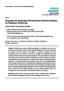
the colony are carried out without centralized control. A bee colony adapts to dynamic environmental conditions. When ..... ester Bay of Massachusetts (Figure 6).
An Adaptive, Scalable and Self-Healing Sensor Network Architecture for Autonomous Coastal Environmental Monitoring Pruet Boonma and Junichi Suzuki Department of Computer Science University of Massachusetts, Boston {pruet, jxs}@cs.umb.edu Abstract Wireless sensor networks (WSNs) are key technology enablers for the current and near future security and surveillance systems. In order to build realtime, multi-modal, high resolution monitoring in those systems, WSN applications need to address critical challenges such as autonomy, scalability, self-healing and simplicity. Based on the observation that various biological systems have developed mechanisms to meet these challenges, BiSNET (Biologically-inspired architecture for Sensor NETworks) implements key biological mechanisms such as energy exchange, pheromone emission, replication and migration to design WSN applications. This paper describes major system components in BiSNET and shows recent simulation results to evaluate BiSNET for oil spill detection in the coastal environment. Simulation results show that BiSNET allows sensor nodes to autonomously adapt their node states and data transmission according to dynamic changes in node/network conditions, retain their power efficiency against the increase of network size (up to 600 nodes), and collectively self-heal (i.e., detect and eliminate) false positive sensor data. Thanks to a set of simple biologically-inspired mechanisms, the BiSNET runtime is implemented lightweight.
1. Introduction Wireless sensor networks (WSNs) are key technology enablers for the current and near future security and surveillance systems. In order to build realtime, multi-modal, high resolution monitoring in those systems, WSN applications need to address critical challenges such as autonomy– the ability to operate in an unattended (and possibly hostile) area with the minimal aid from base stations and human administrator [1, 2]; scalability–the ability to scale to, for example, a large number of sensor nodes1 and a large amount of data generated by sensor nodes [1, 3]; adaptability–the ability to adapt to dynamic conditions of WSNs (e.g., network traffic and resource availability) and sensor nodes (e.g., sensor readings and power consumption) [3, 4, 5]; self-healing–the ability to detect and eliminate false positive data from miscalibrated/malfunctioning 1 For example, the DARPA Networked Embedded Systems Technology program envisions networks consisting of 100 to 100,000 sensor nodes.
nodes [6]; and simplicity–design simplicity and lightweight in footprint due to resource constraints in sensor nodes. The authors of the paper observe that various biological systems have already developed the mechanisms to overcome the above challenges [7]. For example, bees act autonomously, influenced by local environmental conditions and local interactions with other bees. A bee colony can scale to a massive number of bees because all activities of the colony are carried out without centralized control. A bee colony adapts to dynamic environmental conditions. When the amount of honey in a hive is low, many bees leave the hive to gather nectar from flowers. When the hive is full of honey, bees rest in the hive or expand the hive. Also, bees recover (or self-heal) their pheromone traces to flowers when a part of them is lost. The structure and behavior of each bee are very simple; however, a group of bees autonomously emerges desirable system characteristics such as adaptability and self-healing through collective behaviors and interactions among bees. Based on this observation, the proposed framework, called BiSNET (Biologically-inspired architecture for Sensor NETworks), applies key biological principles and mechanisms to design WSN applications. The BiSNET runtime consists of two software components: agents and middleware platforms (Figure 1), which are modeled as bees and flowers, respectively. Each WSN application is designed as a decentralized collection of multiple agents. This is analogous to a bee colony (application) consisting of multiple bees (agents). Agents follow key biological principles such as decentralization, autonomy, food gathering/consumption and natural selection. They collect sensor data (nectars) on platforms (flowers) atop sensor nodes, and carry the data to base stations, which are modeled as nests for bees. Agents perform these functionalities by autonomously invoking biological behaviors such as pheromone emission, replication, reproduction, migration. A middleware platform runs atop of TinyOS in each sensor node, and hosts one or more agents. It controls the state of the underlying node (e.g., sleep and listen states), gather necessary information for node localization and transmit it to a base station, and provides runtime services that agents use to perform their functionalities and behaviors.
Figure 1. BiSNET Runtime Architecture
Figure 2. A Sample WSN Organization
This paper focuses on three major system components in BiSNET: the BiSNET runtime, the node localization mechanism in BiSNET and the BiSNET GUI. This paper also shows recent simulation results to evaluate BiSNET for oil spill detection in the coastal environment. Simulation results show that BiSNET allows sensor nodes to autonomously adapt their node states and data transmission according to dynamic changes in node/network conditions, retain their power efficiency against the increase of network size (up to 600 nodes), and collectively self-heal (i.e., detect and eliminate) false positive sensor data. Thanks to a set of simple biologically-inspired mechanisms, the BiSNET runtime is implemented lightweight.
sors5 , salinity sensors6 and temperature sensors7 ) detects and monitors the spill. Oil may move and spread fast, change the direction of movement, and split into multiple chunks. Some chunks may burn, and others may evaporate and generate toxic fumes. The WSN provides real-time sensor data so that human operators can efficiently dispatch first responders to contain spilled oil in the right place at the right time, and avoid secondary disasters by directing nearby ships to move away from the oil, alerting nearby facilities or evacuating people from nearby beaches. In-situ WSNs can deliver more accurate information (sensor data) to operators more rapidly than visual observation does from the air or coast. Also, in-situ WSNs are less expensive than radar observation with aircrafts or satellites [13].
2. A Motivating WSN Application
3. The BiSNET Runtime
BiSNET operates on a multi-modal WSN2 , which consists of battery-operated sensor nodes and several base stations. BiSNET currently assumes that all nodes are stationary and base stations are equipped with GPS devices. Base stations are linked to the gateway that in turn connects to a backend database and GUI for human administrators (Figure 2). When an agent arrives a base station, it stores the sensor data it carries to a database. BiSNET is intended to be used for oil spill detection and monitoring in the coastal environment. Oil spills occur frequently3 and have enormous impacts on maritime/on-land businesses, nearby residents and the environment. When an oil spill occurs due to, for example, broken equipment of an oil tanker and coastal oil station, illegal oil dumping or terrorism, an in-situ WSN of fixed buoy-attached sensor nodes (e.g., fluorometers4, surface roughness sen-
This section presents the design of the BiSNET runtime.
3.1. BiSNET Agent In BiSNET, agents are decentralized. There are no centralized entities to control and coordinate agents. Decentralization allows agents to be scalable by avoiding a single point of performance bottlenecks and failures [14, 15]. Each agent consists of attributes, body and behaviors. Attributes carry descriptive information on an agent. They include agent type (e.g., fluorescence sensing agent and water roughness sensing agent), sensor data to be reported to a base station, time stamp of the sensor data, and ID/location of a sensor node where the sensor data is captured. Body implements the functionalities of an agent: collecting and processing sensor data (e.g., discarding it or reporting it to a base station). Depending on their agent types, different agents collect different types of sensor data. Behaviors implement actions inherent to all agents. Similar to biological entities (e.g., bees), agents sense their local and surrounding environment conditions, and behave ac-
2 A multi-modal WSN deploys multiple types of sensor nodes. Data from different types of nodes are aggregated, through in-network processing, to provide a multi-dimensional view of collected data. 3 The US Coast Guard reports that 50 oil spills occurred in the US shores in 2004 [8], and the Associated Press reported that, on average, there was an oil spill caused by the US Navy every two days from fiscal year 1990 to 1997 [9] 4 Fluorescence is a strong indication of the presence of oils. Certain compounds in oil absorb ultraviolet light, become electronically excited and fluoresce [10]. Different types of oil yield different fluorescent intensities (emission wavelengths) [11].
5 Oil films locally damp sea surface roughness and give dark signatures, so-called slicks [10]. 6 Water salinity influences whether oil floats or sinks. Oil floats more readily in salt water. It also affects the effectiveness of dispersants [12]. 7 Water temperature impacts how fast oil spreads. Oil spreads faster in warmer waters than in cold waters [12].
2
tion periodically propagates base station pheromones, whose concentration decays on a hop-by-hop basis. Using base station pheromones, agents can approximate where base stations exist, and move toward the base stations by climbing pheromone gradients.
cording to the conditions without any intervention from/to other agents, platforms, base stations and human administrators. This paper focuses on the following five behaviors. (1) Food gathering and consumption: Biological entities strive to seek food for living. For example, bees gather nectar and digest it to produce honey. In BiSNET, agents (bees) read sensor data (nectar) in each duty cycle, and digest it to energy (honey)8. (Energy gain is proportional to an absolute change between the current and previous sensor data.) Agents periodically deposit some of their energy units to their local platforms, and keep the rest for living. (2) Pheromone emission: Agents may emit different types of pheromones (replication and migration pheromones) according to their local and surrounding network conditions. Agents emit replication pheromones in response to the abundance of stored energy (i.e., significant changes in their sensor readings). Different types of agents emit different types of replication pheromones, each of which carries sensor data. For example, on fluorometers, agents emit replication pheromones that contain fluorescence spectrum (fluoro-pheromones). On infrared sensors measuring surface roughness, agents emit replication pheromones that contain surface roughness data (roughness pheromones). Replication pheromones stimulate the agents on the local and one-hop away nodes to replicate themselves. On the other hand, agents emit migration pheromones on their local nodes when they migrate to neighboring nodes. Each pheromone has its own concentration. The concentration decays by half at each duty cycle. A pheromone disapears when its concentration becomes zero. (3) Replication: Agents may make a copy of themselves in response to the abundance of energy and replication pheromones. Each agent does not initiate replication until enough types of replication pheromones become available on the local node. For example, an agent may replicate itself only when both a roughness pheromone and fluoropheromone are available. A replicated (child) agent retains the same agent type as its parent’s type, and aggregates multiple sensor data stored in multiple replication pheromones. A child agent is placed on the platform that its parent resides on, and it receives the half amount of the parent’s energy level. Each child agent is intended to move toward a base station to report aggregated sensor data. (4) Migration: Agents may move from one sensor node to another in response to energy abundance (i.e., significant changes in their sensor readings). Migration is used to transmit agents (sensor data) to base stations. Each agent may implement one of or a combination of the following three migration policies:
• Chemotaxis: Agents may follow migration pheromone traces on which many others travel. These traces can be the shortest paths to the base stations. When no migration pheromones exist on neighboring nodes, agents perform directional walk. • Detour walk: Each agent may go off a migration pheromone trace and follow another path to a base station when the concentration of migration pheromones is too high on the trace (i.e., when too many agents follow the same migration path). This avoids separating the network into islands. The network can be separated with the migration paths that too many agents follow, because the nodes on the paths consume more power than others and they go down earlier than others. In addition to the detour with migration pheromones, agents may avoid moving through the nodes where the concentration of replication pheromones is too high (i.e., where agents detect significant changes in their sensor readings). This detour walk distributes power consumption of agent migration over the nodes where agents detect no changes in their sensor readings, thereby avoiding the network to be separated. (5) Death: Agents expend a certain amount of energy to perform their behaviors. (The energy costs to invoke the behaviors are constant for all agents.) Agents die due to lack of energy when they cannot balance energy gain and expenditure. When an agent dies, the local platform removes the agent and releases all resources allocated to the agent. while true Read sensor data and convert the data to energy(EF ). Update energy level (E(t)) if E(t) < death threshold (TD ) then Invoke the death behavior. if E(t) > replication pheromone emission threshold (TP ) then Emit a replication pheromone. while E(t) > replication threshold(TR ) and replication pheromone concentration(Pi ) > stimulation threshold (TSi ) do n Make a child agent. do Give the half of the current energy level to the child agent. Deposit energy units (EP ) to the local platform. if the local platform is in the broadcast state ( if # of agents n in the local platform > 1 Place a migration pheromone on the local node. then then Move to a neighboring node.
Figure 3. Agent Actions in Each Duty Cycle
• Directional walk: Each agent may move to the nearest base station through the shortest path. Each base sta-
Figure 3 shows a sequence of actions that each agent performs in each duty cycle. First, an agent reads sensor data (as nectar) with the underlying sensor device, and converts it to energy (honey). The energy intake (EF ) is calculated
8 The concept of energy in BiSNET does not represent the amount of physical battery in a sensor node. It is logically affects agent behaviors.
3
the other half. ER is the cost (energy units) for an agent to invoke the replication behavior. A replicated (child) agent aggregates the sensor data in the pheromones that stimulated its parent agent to perform a replication. Agents replicate themselves only when they gain a large amount of energy on the local node and receive enough types of high-concentration pheromones from the local and neighboring nodes. This means that sensor data are aggregated and transmitted to base stations only when significant changes in sensor data are detected on the local and neighboring nodes. Agents do not respond to minor changes in their sensor readings (e.g., water temperature changes during a day or between seasons). This reduces power consumption in sensor nodes and expands the network lifetime by avoiding unnecessary data transmissions. This adaptive data aggregation and transmission mechanism are designed with a self-healing capability in mind, which allows agents to detect and eliminate false positive sensor data. When a node does not work properly due to, for example, malfunctions or miscalibrations, each agent on the node emits the replication pheromones that contain false positive sensor data. A large number of false positive pheromones may be transmitted to neighboring nodes. However, they are discarded at the neighboring nodes because they are not aggregated with other types of pheromones. This means that false positive pheromones are not propagated more than two hops from a malfunctioning or miscalibrated node. Also, agents stop emitting false positive pheromones on the malfunctioning/miscalibrated node because their pheromone emission thresholds increase. Each agent deposits a certain amount of energy (EP ) to a platform that it resides on (see also Figures 3): n
with Equation 1. S denotes the absolute difference between sensor data in the current and previous duty cycles. M is the metabolic rate, which is a constant between 0 and 1. EF = S · M
(1)
Given EF , each agent updates its energy level as follows. E(t) = E(t − 1) + EF
(2)
E(t) is the current energy level of the agent, and E(t−1) is the agent’s energy level in the previous duty cycle. t is incremented by one at each duty cycle. If an agent’s energy level (E(t)) becomes very low (below the death threshold: TD ), the agent dies due to energy starvation (see also Figure 3)9 . An agent emits a replication pheromone if its energy level exceeds its emission threshold TP (Figures 3). Each agent continuously adjusts its TP as the EWMA (Exponentially Weighted Moving Average) of its energy level (E): TP (t) = (1 − α)TP (t − 1) + αE(t)
(3)
TP (t) is the current replication pheromone emission threshold, and TP (t − 1) is the one in the previous duty cycle. EWMA is used to smooth out short-term minor oscillations in the energy level of an agent (E). It places an emphasis on the long-term transition trend of E; only significant changes in E affects TP . α is a constant to control the sensitivity of TP against the changes of E. When a replication pheromone is emitted on a node, all the agents on the node can sense it. An agent replicates itself when it meets two condition: (1) when the agent’s energy level (E(t)) exceeds its replication threshold (TR ), and (2) when the concentration of each type of available replication pheromones (Pi 10 ) exceeds its stimulation threshold TSi (Figures 3). The agent keeps replicating itself until its energy level becomes less than its TR . Agents continuously adjust their replication thresholds as the EWMA of their energy levels (Equation 4). The stimulation threshold of a replication pheromone changes as the EWMA of the pheromone’s concentration (Equation 5). TR (t) = (1 − β)TR (t − 1) + βE(t) TSi (t) = (1 − γ)TSi (t − 1) + γPi (t)
EP =
E(t) − E(t − 1) 0
if E(t) ≥ E(t − 1) if E(t) < E(t − 1)
(6)
Each agent strives to keep its energy level (E(t)) close to the one in the previous duty cycle (E(t P − 1)). When a platform’s total energy gain ( EP ) is greater than a threshold (TB ), the platform changes its state to the broadcast state. This allows agents and pheromones to move to neighboring platforms (see also Figures 3)11 . Each agent uses Equation 7 to determine which node it migrate to when there are multiple neighboring nodes. 3 X Pt,j − Pt
(4) (5)
TR (t) is the current replication threshold. TSi is the current replication pheromone stimulation threshold for the replication pheromone type i. β and γ are the constants to control the sensitivity of TR and TSi against the changes of E and Pi , respectively. A replicating (parent) agent splits its energy units to R ), gives a half to its child agent, and keeps halves ( E(t)−E 2
W Sj =
wt
t=1
min
Ptmax − Ptmin
(7)
Each agent calculates this weighted sum (W S) for each neighboring node j, and moves to a node that generates the highest weighted sum. t denotes pheromone type; P1j , P2j and P3j represent the concentrations of base station, mi-
9 If all agents are dying on a platform at the same time, a randomly selected agent will survive. At least one agent runs on each platform. 10 P denotes the total concentration of pheromone type i. i indicates the i type of pheromones (e.g., roughness and fluoro-pheromones).
11 All agents migrate from a platform whose energy gain is greater than TB , except a randomly selected agent. If there is only one agent in a platform, the agent cannot migrate. At least one agent runs on a platform.
4
4. Node Localization in BiSNET
gration or replication pheromones on a neighboring node j. Ptmax and Ptmin are the maximum and minimum concentrations of Pt among neighboring nodes. wt is used to specify which migration policies each agent performs. w2 and w3 are zero for agents performing directional walk. w2 is positive and negative for agents performing chemotaxis and the detour walk with migration pheromones, respectively. w3 is negative for agents performing the detour walk with replication pheromones.
BiSNET implements its own localization mechanism that approximates the physical locations of individual nodes by using base stations as reference points. Note that each base station keeps track of its location with a GPS device (see Section 2). The proposed localization mechanism is an extension to the Hop-TERRAIN and Refinement algorithms [16]. The mechanism consists of two phases: network distance measurement, which individual nodes perform, and location approximation, which the gateway performs.
3.2. BiSNET Platform Each platform consists of three parts: runtime services, localization support unit and state controller. Runtime services hide lower-level computing and networking details, and provide high-level services that agents use to read sensor data and perform behaviors (see Figure 1). Localization support unit collects the information necessary for node localization (e.g., the distances to base stations), and transmits the information to the gateway via base stations (see also Figure 2). See Section 4 for more details on how the gateway localizes sensor nodes. State controller changes the state of a node to control its sleep period. Each node can be in the listen, broadcast or sleep state. A platform and agents can work on a node when its state is in the listen or broadcast state. In either state, each agent performs the actions described in Figure 3.
4.1. Network Distance Measurement This phase is to measure the topological distances (network hop counts) between each node and base stations. When a base station periodically propagates a base station pheromone (see Section 3.1), the pheromone contains its ID, its concentration and a hop count from the base station. The concentration decays on a hop-by-hop basis. The hop count is initialized as zero and incremented on a hop-byhop basis. When a node receives a base station pheromone, the platform on the node extracts the information from the pheromone, and forwards it to neighboring nodes except the sender of the pheromone. Each platform maintains a base station table, which keeps the shortest distance (hop count) to each base station and the neighboring node through which the platform can reach each base station in the shortest path. Each platform also maintains a neighboring node table, which records the data transmission latency to each neighboring node. When a platform receives a base station pheromone, it compares the hop count in the pheromone with that in its base station table. If the hop count in the pheromone is less than that in the table, the table is updated to record the hop count in pheromone. Otherwise, the pheromone is discarded. (It is not forwarded to neighboring nodes.) The platform also updates its neighboring node table with the transmission latency of a base station pheromone. When a base station receives a base station pheromone from another base station, it performs the same operations as described above. In a particular interval after propagating base station pheromones, each base station propagates inquiry messages to sensor nodes on a hop-by-hop basis. When a node receives an inquiry message, the platform on the node returns its two tables (base station table and neighboring node table) to the closest base station. When a base station receives the tables, it forwards the tables to the gateway.
Figure 4. Platform State Transition In the listen state, a platform turns on a radio receiver to receive data (agents and pheromones) from neighboring sensor nodes. The listen state changes to the broadcast state ifP a platform gains energy more than the broadcast threshold ( EP > TB ; see also Figures 4). In the broadcast state, a platform turns on a radio transmitter to allow agents and pheromones to move to neighboring nodes. P When a platform gains no energy from agents ( EP = 0), the platform goes into the sleep state (Figure 4). The sleep period is determined as follows. Psleep is a constant, and Pi is the concentration of each type of pheromones (the pheomone type i) available on the platform. ( P P sleep P if Pi > 0 P i sleep period = (8) P Psleep
if
4.2. Location Approximation In this phase, the gateway periodically approximates the physical location of each sensor node based on the table information collected with inquiry messages. This phase consists of three processes: distance approximation, location calculation and location adjustment.
Pi = 0
Each platform increases its sleep period to reduce power consumption when agents find no significant changes in their sensor readings on the local and neighboring nodes.
5
Distance approximation. This process approximates the geographical distances between each node and base stations. Let Bi and Bj be base stations, and let their locations be (Bix , Biy ) and (Bjx , Bjy ). Dij is the geographical distance between Bi and Bj , and Hij is the hop count between Bi and Bj . Let N be the node whose location is being calculated. HiN is the hop count between Bi and N , and HjN is the hop count between Bi and N . The geographical distances between a node and base stations are approximated as follows. DiN and DjN are the distances between N and Bi and Bj , respectively. DiN
=
DjN
=
Dij Hij Dij Hij
× HiN
is performed with every pair of neighboring nodes that have lower standard deviation than the node whose location is being adjusted. The average and standard deviation of the obtained (Nx , Ny ) values is calculated. This process is performed iteratively on all the nodes that have standard deviation over a threshold, from the smallest to the largest.
5. AMBIENT: BiSNET User Interface AMBIENT13 is a web-based interactive GUI system, which is connected to a WSN via base stations. It processes sensor data gathered by agents, and maps/visualizes the data on satellite images so that human administrators can immediately detect, monitor and respond events (oil spills) in observation areas. Currently, AMBIENT superimposes the information that BiSNET gathers (e.g., node location and sensor data) on a satellite image of Google Maps14 . Figure 5 shows an example screenshot of AMBIENT. Circles represent sensor nodes. The size of circles depicts sensor data; larger circles means higher values in sensor data. In this example, there exist two types of sensor nodes, each of them has different color; red for fluorometers and blue for water roughness sensors. The brightness of circles represents the confidence (standard deviation) of node localization; the brighter, the more confident.
(9)
× HjN
Dij /Hij is the estimated geographical distance per hop. Note that each base station’s location is available because it equips a GPS device. Location calculation. This process approximates the location of each node by performing trilateration calculations with the locations of multiple base stations. Given DiN , DjN from Equation 9, the following equations are derived. (Bix − Nx )2 + (Biy − Ny )2 (Bjx − Nx )2 + (Bjy − Ny )2
2 = DiN 2 = DjN
(10)
The following is the subtraction of the second equation from the first one. 2 − B 2 − 2(B Bix ix − Bjx )Nx + jx 2 − B 2 − 2(B 2 2 Biy iy − Bjy )Ny = Din − Djn jy
(11)
Reordering the terms gives the following equation. Ny =
2 − B 2 − 2(B 2 2 2 2 Bix ix − Bjx )Nx + Biy − Bjy − Din − Djn jx
2(Biy − Bjy )
(12)
Nx can be calculated by assigning Equation 12 to Ny in the first line of Equation 10. In the same say, multiple (Nx , Ny ) values are calculated with different pairs of base stations. The average of the values is used as the location of Node N , and the standard deviation is used as the confidence of node localization. Position adjustment. This process adjusts the location of a node when the standard deviation of node localization is greater than a threshold12. This process is similar to the location calculation, but instead of using base stations as reference points, the neighboring nodes who have low standard deviation are used. In addition, data transmission latency is used instead of hop count. This process starts with choosing a node that has the smallest standard deviation beyond a threshold, chooses two neighboring nodes that have lower standard deviation as reference points, and then uses the Equation 12 to adjust the node’s location. This process
Figure 5. A Screenshot of AMBIENT
6. Simulation Results This section shows a set of simulation results to evaluate BiSNET. BiSNET is implemented on TinyOS and evaluated in the PowerTOSSIM simulator. This simulation study emulates a WSN deployed on the sea to detect oil spills (Section 2). The WSN consists of fluorometers and surface roughness sensors randomly deployed in an N xN grid topology. Two different size of WSNs are examined, 25x24 and 8x7. A half of nodes equip fluorometers and the other half equips surface roughness sensors. Four nodes at vertices work as base stations as well 13 AMBIENT (AMBIENT is a Module for BiSNET’s Interactive obsErvation for seNsor neTworks) 14 http://maps.google.com/
12 The
sensor nodes near the borders of a WSN have higher localization errors than the sensor nodes inside a WSN.
6
(Figure 6). This study assumes that 100 barrels (approximately 3,100 gallons) of crude oil is spilled in the Dorchester Bay of Massachusetts (Figure 6). Simulation data set is generated with an oil spill trajectory model implemented in the General NOAA Oil Modeling Environment [17].
Table 2. Average Data Transmission Latency Network size
Average (Second)
Standard Deviation
25x24 8x7 25x24 8x7
54 23 53 23
5 5 4 3.5
GBR BiSNET
6.2. Power Consumption Table 3 shows the average power consumption of sensor nodes throughout a simulation. Power consumption per node is almost same in BiSNET and GBR, although BiSNET operates in a higher temporal resolution than GBR does. The in-network data aggregation of BiSNET reduces network traffic, and in turn power consumption on nodes. The power consumption per reported sensor data is consistently lower in BiSNET than GBR. BiSNET reduces 14% power consumption per reported data. This means that BiSNET manages power consumption effectively while increasing the temporal resolution of data collection. Please also note that the standard deviation of power consumption per node is consistently lower in BiSNET than GBR. This means BiSNET distributes power consumption over more nodes than GBR, thereby reducing a risk of network separation more effectively than GBR.
Figure 6. A Simulated Oil Spill BiSNET is compared with a routing protocol for WSNs, GBR (Gradient Based Routing) [18]. In GBR, a base station periodically propagates a routing message to sensor nodes throughout the network. The routing message gradually assigns smaller gradient hight values to nodes as it travels on a hop by hop basis. Given a gradient toward a base station, each node forwards sensor data to a neighboring node that has a higher gradient hight. In GBR, sensor data is transmitted on the shortest paths to base stations. In BiSNET, agents perform all the behaviors described in Section 3.1, including all three migration policies.
Table 3. Average Power Consumption per Sensor Node and Sensor Data
6.1. Success Rate and Latency
GBR BiSNET
# of reported data
Success rate
25x24 8x7 25x24 8x7
185 105 215 122
180 102 210 120
97.30% 97.14% 97.67% 98.36%
Standard Deviation
Average per Data (mA)
25x24 8x7 25x24 8x7
1546 1035 1544 1038
200 120 168 103
8.6 10.1 7.3 8.7
BiSNET
6.3. Network Lifetime Table 4 shows the network lifetime; how soon sensor nodes go down due to lack of power. Every node has the same limited battery capacity (500 mAh). In GBR, 18 of 600 (25x24) nodes go down in 750 minutes. On the other hand, only 6 nodes go down in BiSNET. BiSNET successfully reduces and distributes power consumption over nodes and expand the network life by taking advantage of its innetwork data aggregation and agent detour walk behavior with migration and replication pheromones.
Table 1. The Total Number of Collected and Reported Sensor Data # of collected data
Average per Node (mA)
GBR
Table 1 shows the total number of sensor data collected and reported to base stations throughout a simulation. Compared with GBR, BiSNET always operate in a higher temporal resolution because of BiSNET’s adaptive management of sleep period (see Equation 8). The increase in the number of reported data is 16.67% in the 25x24 WSN and 17.67% in the 8x7 WSN. Note that the success rate of data transmission is almost same between BiSNET and GBR even if BiSNET operates in a higher temporal resolution.
Network size
Network Size
Table 4. Sensor Node Lifetime GBR
Table 2 shows the average latency to transmit sensor data from nodes to base stations. The latency is almost same in BiSNET and GBR. BiSNET operates in a higher temporal resolution than GBR does; however, it performs in-network data aggregation. This reduces the number of migrating agents, and in turn, network traffic.
BiSNET
Network Size
0-250 minute
250-500 minute
500-750 minute
25x24 8x7 25x24 8x7
2 2 0 0
6 7 1 3
10 10 5 3
6.4. Self-Healing Table 5 shows how the self-healing capability of BiSNET impacts power consumption. BiSNET provides two 7
self-healing capabilities: intra-node and inter-node selfhealing. Intra-node self-healing allows agents to detect that the local node malfunctions and avoid false positive data to be propagated to neighboring nodes. (For example, sensor reading may swing between very low and very high value on a malfunctioning node.) Inter-node self-healing allows agents to detect malfunctions in neighboring nodes and discard false positive data from the node. As Table 5 illustrates, these two self-healing capabilities significantly reduce power consumption by reducing unnecessary data transmissions.
size (up to 600 nodes), and collectively self-heal (i.e., detect and eliminate) false positive sensor data. Thanks to a set of simple biologically-inspired mechanisms, the BiSNET runtime is implemented lightweight.
References [1] M. Yu, H. Mokhtar, and M. Merabti, “A survey of network management architecture in wireless sensor network,” in Proc. of the Sixth Annual PostGraduate Symposium on The Convergence of Telecommunications, Netowrking & Broadcasting, Jun 2006. [2] J. Blumenthal, M. Handy, F. Golatowski, M. Haase, and D. Timmermann, “Wireless sensor networks - new challenges in software engineering,” in Proc. of Emerging Technologies and Factory Automation, September 2003.
Table 5. Average Power Consumption of Each Sensor Node Network Size
Average per Node (mA)
Standard Deviation
25x24 8x7 25x24 8x7
2853 2202 1544 1140
1520 1350 168 152
Without Self-Healing With Self-Healing
[3] S. Hadim and N. Mohamed, “Middleware challenges and approaches for wireless sensor networks,” IEEE Distributed Systems Online, vol. 7, no. 3, pp. 853–865. IEEE, 2006. [4] I. Akyildiz, W. Su, Y. Sankarasubramaniam, and E. Cayirci, “Wireless sensor networks: a survey,” Elsevier Journal of Computer Networks, vol. 38, pp. 393–422, 2002. [5] J. Ledlie, J. Schneidman, M. Welsh, M. Roussopoulos, and M. Seltzer, “Open problems in data collection networks,” in Proc. of European SIGOPS, September 2004.
6.5. Scalability
[6] P. Rentala, R. Musunuri, S. Gandham, and U. Sexena, “Survey on sensor networks,” in Proc of Int’l Conf. on Mobile Computing and Networking, 2001.
In order to evaluate the scalability of BiSNET against the number of nodes and the amount of sensor data collected by nodes, the same set of simulations (see Sections 6.1, 6.2, 6.3 and 6.4) was carried out on the WSNs consisting of 600 (25x24) nodes and 56 (8x7) nodes. The simulation results are qualitatively same in both cases; BiSNET is scalable against the increase of network size and data volume.
[7] T. Seeley, The Wisdom of the Hive. Harvard University Press, 2005. [8] U. C. Guard, “Polluting incident compendium: Cumulative data and graphics for oil spills 1973-2004,” Tech. Rep., September 2006. [9] L. Siegel, “Navy oil spills,” Webpage, November 1998. [10] J. M. Andrews and S. H. Lieberman, “Multispectral fluorometric sensor for real time in-situ detection of marine petroleum spills,” in Proc. of the Oil and Hydrocarbon Spills, Modeling, Analysis and Control Conference, July 1998.
6.6. Simplicity: Memory Footprint Table 6 shows the memory footprint of the BiSNET runtime in a MICA2 mote, and compares it with the footprint of Blink (an example program in TinyOS), which periodically turns on and off an LED, GBR, and Agilla, which is a mobile agent platform for WSNs [19]. The BiSNET runtime is lightweight in its footprint thanks to the simplicity of the biologically-inspired mechanisms in BiSNET.
[11] C. E. Brown, M. F. Fingas, and J. An, “Laser fluorosensors: A survey of applications and developments,” in Proc. of the Twenty-forth Arctic and Marine Oil Spill Program Technical Seminar, June 2001. [12] U. E. P. Agency, “Understanding oil spills and oil spill response,” Tech. Rep., 1999. [13] M. F. Fingas and C. E. Brown, “Review of oil spill remote sensors,” Spill Science & Technology Bulletin Journal, vol. 4, no. 4, pp. 199– 208, 1997.
Table 6. Memory Footprint in a MICA2 Mote BiSNET Blink GBR Agilla
ROM (KB)
RAM (KB)
1.0 0.04 0.84 3.59
24 1.6 26 41.6
[14] R. Albert, H. Jeong, and A. Barabasi, “Error and attack tolerance of complex networks,” Nature, vol. 406, July 2000. [15] N. Minar, K. H. Kramer, and P. Maes, “Cooperating mobile agents for dynamic network routing,” Software Agents for Future Communications Systems. Springer, 1999. [16] C. Savarese, J. Rabay, and K. Langendoen, “Robust positioning algorithms for distributed ad-hoc wireless sensor networks usenix technical annual conference,” in Proc. of USENIX Technical Annual Conference, June 2002.
7. Conclusion
[17] C. Beegle-Krause, “General NOAA oil modeling environment (GNOME): A new spill trajectory model,” in Proc. of Internation Oil Spill Conference, March 2001.
This paper describes a biologically-inspired architecture, called BiSNET, which coherently applies a small set of simple biological concepts to design WSN applications. Simulation results show that BiSNET allows sensor nodes to autonomously adapt their node states and data transmission according to dynamic changes in node/network conditions, retain their power efficiency against the increase of network
[18] C. Schurgers and M. Srivastava, “Energy efficient routing in wireless sensor networks,” in Proc. of MILCOM 2001, 2001. [19] C.-L. Fok, G.-C. Roman, and C. Lu, “Rapid development and flexible deployment of adaptive wireless sensor network applications,” in Proc. of Int’l Conf. on Distributed Computing Systems, June 2005.
8