An Adaptive Sensor Mining Model for Pervasive Computing Applications Parisa Rashidi
Diane J. Cook
Washington State University Pullman, WA US, 99164 001-5093351786
Washington State University Pullman, WA US, 99164 001-5093354985
[email protected]
[email protected]
ABSTRACT In the past decade, the fields of pervasive computing, sensor design and data mining have begun to converge. As a result, there is a wealth of sensor data that can be analyzed with the goals of identifying patterns and automating sequences. Mining sequences of sensor events brings unique challenges to the KDD community. The challenge is heightened when the underlying data source is dynamic and the patterns change. In this work, we introduce a new adaptive mining approach that utilizes two cooperating algorithms to detect patterns in sensor event data and to adapt to changes in the underlying model. The first algorithm, the Frequent and Periodic Pattern Miner (FPPM), discovers frequent and periodic event patterns of arbitrary length and inexact periods. Our second algorithm, the Pattern Adaptation Miner (PAM), complements FPPM by detecting changes in the discovered patterns. Our approach also captures vital context information such as pattern triggers and event timings. In this paper, we present a description of our mining algorithms and validate the approach using data collected in our CASAS smart home testbed.
Categories and Subject Descriptors H.2.8 [Database Management]: Database Applications– data mining; I.2.6 [Artificial Intelligence]: Learning– knowledge acquisition; H.4.m [Information Systems]: Information system Applications– Miscellaneous.
General Terms Algorithms, Design, Experimentation, Human Factors.
Keywords Sensor data mining, Sequential mining, Pervasive computing applications, Smart environments, Adaptation.
Permission to make digital or hard copies of all or part of this work for personal or classroom use is granted without fee provided that copies are not made or distributed for profit or commercial advantage and that copies bear this notice and the full citation on the first page. To copy otherwise, or republish, to post on servers or to redistribute to lists, requires prior specific permission and/or a fee. Conference’04, Month 1–2, 2004, City, State, Country. Copyright 2004 ACM 1-58113-000-0/00/0004…$5.00.
1. INTRODUCTION With remarkable recent progress in computing power, networking equipment, sensors, and various data mining and artificial intelligence methods, we are steadily moving towards ubiquitous and pervasive computing, beyond PCs and mobile phones, into a world entangled with sensors and actuators, where technology recedes into the background of our lives. In the past decade, the fields of pervasive computing, sensor design and data mining have begun to converge. As a result, there is a wealth of sensor data that can be analyzed with the goals of identifying patterns and automating sequences. Mining sequences of sensor events brings unique challenges to the KDD community. By discovering repetitive sequences, modeling their temporal constraints and learning their expected utilities, we can intelligently automate a variety of tasks such as computer command sequences, assembly sequences, and other complex activities. In this work, we introduce a new adaptive mining approach that utilizes two cooperating algorithms to detect patterns in sensor event data and to adapt to changes in the underlying model. The first algorithm, the Frequent and Periodic Pattern Miner (FPPM), discovers frequent and periodic event patterns of arbitrary length and inexact periods. Our second algorithm, the Pattern Adaptation Miner (PAM), complements FPPM by detecting changes in the discovered patterns. These patterns usually can be expressed as a set of time ordered sequences, and discovering frequent and periodic patterns among such a set of time ordered data can be achieved by using a sequence mining algorithm tailored to special domain requirements for pervasive computing applications such as smart environments. Some pervasive computing special domain requirements include a unified framework for detecting periodic and frequent patterns, adaptation over the lifetime of the system, utilizing temporal information such as sequence start time and event duration distributions, and capturing startup trigger information. In this work we try to address these special domain requirements. Providing an adaptive approach in our work is a significant advantage over previous sequential mining algorithms applied to pervasive computing applications, which assume the learned model is static over the lifetime of the system. In order to show a tangible application of our algorithms, we will evaluate them in the context of a popular pervasive computing application: smart environments. In recent years, smart environments have been a topic of interest for many researchers who have the goal of automating resident activities in order to achieve greater comfort, productivity, and energy efficiency. A
smart home uses networked sensors and controllers to try to make residents' lives more comfortable by acquiring and applying knowledge about the residents and their physical surroundings. We validate our approach on data generated by a synthetic data generator as well as on real data collected in a smart workplace testbed located on campus at Washington State University. testbed
2. Related Work In pervasive computing applications, such as smart environments, not only it is important to find frequent event patterns or activities, but also those that are the most regular, occurring at predictable periods (e.g., weekly, monthly). If we ignore periodicity and only rely on frequency to discover patterns, we might discard many periodic events such as the sprinklers that go off every other morning or the weekly house cleaning. Therefore we need a unified framework that can simultaneously detect both frequent and periodic activity patterns. There are a number of earlier works that try to handle periodicity, such as the Episode Discovery (ED) algorithm [12]; however, the problem with ED and most other approaches is that they look for patterns with an exact periodicity, which is in contrast with the erratic nature of most events in the real world. Lee, et al [5] define a period confidence for the pattern, but they require the user to specify either one or a set of desired pattern time periods. In our approach, we do not require users to specify predefined period confidence for each of the periods, as it is not realistic to force users to know in advance which time periods will be appropriate. In addition, the periodicity of patterns for many practical applications is dynamic and change over time as internal goals or external factors change. In contrast we define two different periodicity temporal granules, to allow for the necessary flexibility in periodicity variances over two different levels. A fine grained granule is defined for hourly periods which can span several hours up to 24 hours, and a coarse grained granule is defined for daily periods which can span any arbitrary number of days. None of these periodicity granules require a period to be exact: fine grained periods provide a tolerance of up to one hour and coarse grained periods provide a tolerance of up to one day.
subsequences by attempting to load up the candidate set with as many candidate sequences as possible before each scan. In our work, we do not combine candidate sequences to generate an exponential number of new candidates, rather we only extend sequences that made the cutoff in the previous iteration by one event that occurs before or after the current sequence, though sliding a window over found sequences. An important issue in sequence mining algorithms is how to determine the window size that slides over data to discover patterns. Several potential solutions to this problem have been proposed such as a maximum allowed inter-node time constraint which dynamically alters window widths based on the lengths of episodes being discovered [7]. Similarly, expiration time constraints may be incorporated in the non-overlapped and non-interleaved occurrence based counts [4]. However, in our case, as we are dealing with overlapped irregular inter-node time constraints, no maximum inter-node time can be determined and therefore the above solutions can not be applied. Instead, we apply a variable-size window whose length increases incrementally. FPPM continues to increase the window size until no frequent or periodic sequences within the new window size are found. This is an improvement over previous versions of smart home data mining techniques such as the ED algorithm [12] which were trying to find frequent sequences in a window of fixed maximum length.
Our work is based on a variant of the Apriori algorithm. The Apriori algorithm attempts to find repeating subsequences, as frequent as at least a minimum occurrence ratio. Apriori sequence mining uses a bottom up approach, where frequent subsequences are extended one item at a time in a step known as candidate generation, and then groups of candidates are tested against the data. The algorithm terminates when no further successful extensions are found that meet the frequency criteria.
A significant source of information in some pervasive computing applications such as smart environments is the contextual information that describes features of the discovered sequence. Context information is valuable for better understanding the patterns and potentially automating them. In our algorithms we will capture context information consisting of startup triggers, event durations, and start times. Most previous techniques treat events in the sequence as instantaneous. In addition, they typically do not differentiate between sensor data (startup triggers) and actuator data, which represents vital contextual information. Laxman and Sastry [4] do model some temporal information, by incorporating event duration constraints into the episode description. A similar idea in the context of sequential pattern mining is proposed by Lee et al. [5], where each item in a transaction is associated with a duration time. Based on the Apriori algorithm, Bettini et al. [2] also have proposed a framework for the discovery of frequent time sequences, placing particular emphasis on the support of temporal constraints on multiple time granularities where the mining process is modeled as a pattern matching process performed by a timed finite automaton. Our work is different from these previous approaches, as we mostly focus on estimating time distributions for different time granules by utilizing combinations of local Gaussian distributions for modeling temporal information of each pattern, rather than merely considering temporal granules. Using a combination of multiple Guassian and several temporal granules allows us to more accurately express and model duration and start times. In our work, we provide the basis for calculating both duration and start time distributions for discovered activity patterns. Additionally, we incorporate startup triggers into our data mining approach to obtain a more powerful representation of activity data in smart environments.
The Apriori algorithm, while historically significant, suffers from a number of inefficiencies or trade-offs, which have spawned other algorithms. Candidate generation creates a large numbers of
One crucial issue that still has not been explored by the sensor mining and smart environment research communities is how to adapt to the changing environment, as events change their
To find frequent patterns, we exploit a subset of the temporal knowledge discovery field, that usually is referred to as “discovery of frequent sequences” [12], [9], “sequence mining” [1] or “activity monitoring” [3]. In this area, the pioneering work of Agrawal, the Aprori algorithm [1], was the starting point, and since then, there have been a number of extensions and variations on the Apriori algorithm, such as parallel episodes detection [6].
patterns in real world situations. This is especially true in the case of smart environments, because humans often change their habits and lifestyle over time. We try to address this issue by using the PAM algorithm to discover any changes in the resident’s lifestyle.
3. MODEL DESCRIPTION We assume that the input data is a sequence of individual event tuples. Each tuple appears is in the form where di denotes a single data source like a motion sensor, light sensor, or appliance; vi denotes the state of the source such as on or off; and the timestamp, ti, which denotes the occurrence time for this particular event. In our context we refer to every individual tuple as an “event” and we will call a sequence of these events a “pattern”, a “sequence”, or to emphasis smart environment applications, an “activity”. We also assume that data is not in stream format, rather it is sent to a storage media, and the data mining process is carried out offline at regular time intervals such as weekly. Table 1 shows a sample of collected data in this format. Table 1 Sample of collected data. Source
State
Timestamp
Light_1
ON
05/15/2007 12:00:00
Light_2
ON
05/15/2007 12:02:00
Motion_Sensor_1
ON
05/15/2007 12:03:00
In the first iteration, a window of size ω (initialized to 2) is passed over the data and every sequence of length equal to the window size is recorded together with its frequency and initial periodicity. Frequency is the number of times the sequence occurs in the dataset, and periodicity is the regularity of occurrence, such as every three hours or weekly. After the initial frequent and periodic sequences have been identified, FPPM incrementally builds candidates of larger size. Instead of combining candidate sequences and scanning the data again, FPPM extends sequences that made the cutoff in the previous iteration by one event that occurs before or after the current sequence. This approach represents a significant efficiency improvement over the Apriori algorithm which generates an exponential number of new candidate patterns in each iteration. FPPM continues to increase the window size until no frequent or periodic sequences within the new window size are found. To provide more efficient access to sequences, the discovered sequences are stored in a hash table. As mentioned earlier, our sequence mining approach also provides the option to detect changes in discovered patterns. There are two options for detecting changes in discovered patterns. First, a fast demand-based option called explicit request allows users to highlight a number of activities to be monitored for changes. Second, a slower automatic option called smart detection automatically looks for potential changes of all patterns, based on a regular mining schedule. The explicit request mechanism detects changes in specified patterns, such that whenever a pattern is highlighted for monitoring, the adaptation algorithm collects data and mines it to find potentially-changed versions of a specific pattern. These changes may consist of new activity start times, durations, triggers, periods, or structure.
Structure change is detected by finding new patterns that occur during the times that we expect the old pattern to occur. Other parameters values are changed if a pattern matches the structure of the highlighted pattern, but has other different parameters (e.g., timing, triggers) have changed. All changes above a given threshold will be considered as different versions of the pattern and will be shown to the user through our user interface. In addition, our smart detection mechanism automatically mines collected data at periodic intervals (e.g., every three weeks) to update the activity model. The smart detection method adapts slower than the explicit request method; however it removes the burden of specifying activities to be monitored. We will next describe these algorithm steps in more detail.
3.1 Basic Frequent Pattern Finding The algorithm finds frequent patterns by visiting the data iteratively where the number of iterations depends on the length of the longest frequent (or periodic) sequence. In the first pass, the whole data is visited to calculate initial frequencies and periods, and in the next passes only a small portion of data is revisited. In the first pass, a window ω of size 2, is slid through the entire input data and every sequence of length ω, denoted by siω along with its frequency, fs, is recorded. Here, the sequence length is equal to the window size ω and i refers to a unique sequence identifier. The frequency fs, of each sequence siω refer to the number of times siω is encountered in the data. In order to mark a sequence as a frequent sequence, its frequency should satisfy certain conditions. Drawing on results from information theory, we evaluate the frequency of a sequence based on its ability to compress the dataset, by replacing occurrences of the pattern with pointers to the pattern definition [8]. Calculating this compression is tricky for smart home data, as the size of the dataset may not be fixed due to varying activity levels (e.g. an active day will generate a lengthy event data stream). Therefore, we compute compression according to Equation 1, where fa represents the frequency of sequence s, t represents the input data length in hours and C represents the compression threshold.
a ∗ fs t
>C
(1)
Previous approaches [2] have calculated the input data length in numbers of tuples, rather than in units of time, which results in making discovery of frequent patterns dependent on the resident’s activity level. For example, if the resident has a very active day, the input data will contain more tuples and therefore the input length will take on a high value, but if resident is not active that day, the input length will have a low value. Therefore for an activity with the same frequency such as making coffee twice a day, the compression value will be dependent on the resident’s activity level. In our approach, the input length is measured in time units rather than tuples, and an activity such as making coffee twice a day will be discovered as a frequent pattern, independent of the activity level of the resident. However there might be an extreme case where the activity level of the resident is below the expected level, which results in the compression values of most or all of the sequences falling below the compression threshold. To adapt to this unexpected situation, we set the compression threshold to the following value where favg
represents the average frequency of all sequences, A represents the average length of sequences whose frequency is above favg, and t is the input data length in hours.
C=
A ∗ f avg
(2)
t
Applying these conditions together helps to avoid marking transient patterns as frequent patterns, while also finding patterns that are frequent independent of the resident’s activity level.
3.2 Basic Periodic Pattern Finding In addition to finding frequent patterns, FPPM is also able to discover periodic patterns. Calculating periods is a more complicated process. To calculate the period, every time a sequence s is encountered, we will compute the elapsed time since its last occurrence. More precisely, if we denote the current and previous occurrence of a sequence pattern as s and sp, and their corresponding timestamps as t(s) and t(sp), then the distance between them is defined as t(s) - t(sp). This distance is an initial approximation of a candidate period. To determine periodicity, as mentioned before, two different periodicity granules are considered: coarse grained and fine grained period granules. A fine grained granule is defined for hourly periods which can span several hours up to 24 hours, and a coarse grained granule is defined for daily periods which can span any arbitrary number of days. None of these periodicity granules require a period to be exact, fine grained periods provide a tolerance of up to one hour and coarse grained periods provide a tolerance of up to one day. One can claim that only a fine grained period can be sufficient to show periodicity of an activity; for example, every Sunday can be represented by a period of 7 × 24 hours instead of a coarse period of 7 days. This claim is not substantiated in practice, as taking such an approach will require the activity to happen every 7 × 24 hours with a tolerance of just 1 hour. But this is not a realistic assumption, as we want to allow for more tolerance in coarse grained periods. For example, consider the scenario when a resident might watch TV every Sunday, but at different times; in this case, a fine grained period is not able to catch periodicity as its tolerance is just one hour while a coarse grained period is easily able to catch such a periodicity as it allows for a tolerance of up to one day. The same claim can be made about other time granules, but for sake of simplicity and demonstrating the basic idea, we will just consider the two levels of temporal granules. To construct periods, a lazy clustering method is used. As long as an activity's period can be matched with previous ones (with a tolerance of one hour for fine grained and one day for coarse grained), no new period is constructed. If the new activity has a period different other than previous periods, a new period is constructed and is added to the tentative list of fine grained or coarse grained periods. In order to make sure that candidate periods are not just some transient accidental pattern, they are kept in a tentative list until they reach a confidence frequency value. If the periodicity for a sequence is consistent a threshold number of times, the pattern is reported as periodic, then it is moved to the consolidated period list. Updating tentative and consolidated lists is performed dynamically and a period can be moved from one list to another several times. Such a schema helps to eliminate any transient periods based on current or future evidence, resulting in an adaptive evolvable mining approach. In
this approach, whenever more data becomes available as a result of regularly scheduled mining sessions, the periods are revisited again, and if there is any period that does not meet periodicity criteria anymore, it will be moved from the consolidated list into the tentative list. Later if we find again more evidence that this period can be consolidated, it will be moved back into the consolidated list. This approach results in a more robust model that can evolve and adapt over time. In the following sections, we will describe in more detail how changes in patterns are discovered and are incorporated into the model. In contrast to frequent pattern finding which uses a single frequency (compression) threshold for detecting all frequent sequences, we can not use a single confidence threshold for detecting all periodic sequences. Rather we need to tailor the confidence threshold to each specific periodic pattern, because the number of times that an activity occurs can vary depending on its period, making a low frequency sequence a valid periodic candidate in some cases, and a relatively high frequency sequence an invalid candidate in other cases. For example, consider a scenario where our input file contains two weeks of resident activity data and there are two periodic activities: a1 with a period of one hour and a2 with a period of 4 days. In this scenario, the number of times we expect to see a1 would be much more than a2. Therefore, a single confidence value can not work for both cases. To work around this problem, as we scan through the data we calculate and update the expected number of occurrences, E(fa), for an activity a, up to current point in data. For example, if our initial period estimate for activity a is 5 hours and so far we have scanned through 10 hours of data, we expect to see two occurrences of activity a in an ideal case. Considering the erratic nature of real-world events, not all sequences will be repeated ideally. To deal with this problem, for each new occurrence of a we check it against the following equation where fa is actual number of occurrences observed so far and ζ is a predefined threshold that determines what percentage of expected occurrences is sufficient to move a candidate periodic sequence from tentative list into consolidated list.
E( f a ) >ζ fa
(3)
The predefined threshold can be different for coarse grained and fine grained periods, which we denote as ζf and ζc. In the next section, we will describe in more detail how the iterative model constructs sequences of larger sizes from basic sequences.
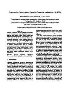
3.3 Iterative Model Construction After the initial frequent and periodic sequences of length two have been identified in the first iteration, the next iteration begins. In later iterations, FPPM does not revisit all the data again. Instead, the algorithm attempts to extend the window by one event to the left and right (before and after) of the discovered frequent or periodic sequences and determines if the extended sequences again satisfy the periodicity or frequency criteria. FPPM thus identifies frequent and periodic sequences of increased length, and continuing this process results in generation of a multi hash-table structure where each member hash table holds all discovered sequences of equal size (see Figure 1).
overall number of 2m extensions at each step, where m is the number of discovered sequences in previous iteration. This approach represents a significant efficiency improvement over the Apriori algorithm which generates an exponential number of new candidate sequences at each iteration. In order to allow for fast retrieval of sequences during window extension, FPPM also maintains an index table for each discovered sequence that points to the locations of all instances of that particular pattern.
3.4 Startup Trigger Information
Figure 1 Multi-hash structure. Incrementing the window size will be repeated until no more frequent (periodic) sequences within the new window size are found. At iteration n, with a window of size n+1, if all occurrences of a sequence a are of length n+1, then the smaller size sequences which were discovered in previous iterations and are subsequences of pattern a will be discarded. This results in correct identification of the maximal sequence, while discarding redundant subsequences. The symmetric expansion of window allows for patterns to grow both forward and backward in time, and the incremental expansion allows for discovery of variablelength patterns. The pseudo-code for the FPPM algorithm is shown in Figure 2.
An important notion that can be used to improve activity prediction in real world data mining applications such as smart environments is the discovery of sequence triggers. Basically, a trigger is an event which consistently causes an activity to start. It can be thought of as a rule composed of a condition and a consequence, such that: trigger → activity. So far, we assumed that each activity can happen either at repeatable periods or frequently at irregular times. However, an activity also can be started whenever it is triggered by other events. For example, in a smart environment, running out of milk in your refrigerator can be a trigger to initiate a supermarket purchase reminder. If we ignore the trigger concept, a set of frequent and periodic sequences will be obtained regardless of whether the events in these patterns are triggers or normal events. However, from a practical point of view, a trigger is an external observable event and should not be considered as part of an automation policy. Instead, it should be considered as a startup condition for frequent or periodic sequences. Therefore it is necessary to augment the data mining model with a trigger processing component that is able to recognize triggers that occur in the observed data. We adopt the following policy for processing triggers:
Figure 2 Psuedo-code for FPPM algorithm. This approach provides a more efficient method for discovering sequences than the original Apriori algorithm, as it does not scan the whole data in each iteration. To elaborate more, consider iteration n-1 where candidates of length n will be generated. Apriori generates candidate sequences by considering all different combinations of previous candidates, resulting in an exponential number of generated candidates. In our approach for each discovered sequence of length n-1, only two extensions will be considered, left and right extensions. This results in generating an
If a trigger appears at the beginning of an activity, it should be removed from the beginning of the sequence and rather be considered as the firing condition for that activity. If a trigger appears at the end of an activity, it has no effect on its preceding activities; therefore it only needs to be removed from the sequence. If several triggers occur consecutively, we will just consider the last one, discarding the other ones. If a trigger occurs in the middle of a sequence, we will split the sequence into two sequences where the trigger becomes the firing condition of the second sequence (see Figure 3). If a sequence contains more than one trigger, the above steps are repeated recursively.
Note that we assume that frequency and period would be the same for split sequences as the original sequence; but, the compression value may change as it depends on the sequence’s length. So, the compression value is computed for recently split sequences and if it does not satisfy the frequency criteria, recently split sequences will be removed from the frequent patterns’ list. Also during the sequence splitting process, sequence might reduce to one of the already existent sequences. In this case, one approach is to repeat the data mining process again to find any existing relation between these two sequences (e.g., they might have different periods). However, for the sake of simplicity and also efficiency, we do not mine the data again; rather we will choose the sequence with the highest compression value and simply discard the other.
Figure 3 A trigger causing a sequence to be split.
3.5 Temporal Information In addition to finding frequent and periodic patterns, FPPM records duration and start times of events by processing their timestamps. We calculate only the start time of the first event of an activity, as the start times of other events can be obtained from preceding events’ durations and the first event’s start time. This new source of information is vital in many real world applications including smart environments, as it can be used to determine temporal relationships between individual events or activities. For each single event a timestamp is kept. After all frequent and periodic sequences have been discovered, the sequences will be organized in a Hierarchal Activity Model (HAM) structure which filters out sequences according to two temporal granule levels of day and hour. Figure 4 shows a sample HAM model. Each sequence will be placed in a HAM leaf node according to its day and time of occurrence. For each activity at each node, we describe the start time and the duration of each individual event using a normal distribution. As the figure shows, HAM decomposes activity information in terms of two temporal granules (day of week and time of day) and activity metadata. The activity data itself is represented using a Markov decision process [10]. Our approach automatically constructs a HAM model from FPPM data. HAM captures temporal relationships between events in an activity by explicitly representing sequence ordering in a Markov model.
HAM, we model the start time of the first event of an activity and durations of all events of an activity using a normal distribution. These distributions are stored in the Markov model nodes. Both distributions are updated every time FPPM mines newlygenerated data. If an activity is located in different time/day nodes within the HAM model, multiple Gaussian distributions for that activity will be computed, allowing HAM to more accurately approximate the start time and duration values, by using multiple simple local functions.
3.6 Adaptation Most pervasive computing mining algorithms generate a static model. These approaches assume that once the desired patterns from sensor data have been learned, no changes need to be applied to maintain the model over time. The challenge is heightened when the underlying data source is dynamic and the patterns change. In the case of smart environments, as we know, humans are likely to change their habits and activity patterns over time depending on many factors, such as social relations, seasonal and weather conditions and even emotional states. Therefore, a static model cannot serve the purpose of a long-term solution for a smart environment. Instead, we need to find a way to adapt to the changes that occur over time. As mentioned earlier, there are two options for detecting changes in discovered patterns: the fast explicit request option that allows users to highlight a number of patterns to be monitored for changes; and the smart detection option that automatically looks for potential changes of all patterns, based on a regular mining schedule. For every discovered sequence, the mining system maintains a potential value, Qi, which shows amount of evidence against or for a sequence as being frequent or periodic. The potential value can be increased or decreased through a compensation effect or a decay effect, as will be described. If potential value falls below a certain activity threshold, the sequence is discarded from the model, in other words it will be forgotten. Maintaining a potential value for each discovered sequence can help us distinguish transient changes from long-term changes that still might be accompanied by a noise element. After every mining session, the discovered activities will include a mixture of new and previously-discovered patterns. For new patterns, we simply can add them to the model and initialize their potential value. However, for previous patterns, the situation is more complicated, as there might be changes in start times, durations or startup triggers, or in the absence of any changes, the activity can be the same as before. We will later discuss the case where pattern attributes are changed; but if the pattern shows no changes, then the only thing that needs to be done is to apply compensation effect to potential value by Equation (4). The case where will be discussed later.
Qi = (Qi + α r )
Figure 4 Example HAM model. There have been earlier approaches to modeling durations of states in a Markov decision process such as the approach by Vaseghi [11] in which state transition probabilities are conditioned on how long the current stated has been occupied. In
(4)
In above equation, r denotes the reward value, and α ∈ [0,1] denotes the learning rate which is a small value to imply gradual history-preserving nature of learning as there is no strong evidence or user guidance that a change is a permanent change and not a temporary one. In order to avoid infinite growth of potential, we allow value functions to grow only in the range of [-1...1].
In addition to the compensation effect effect, we also employ a decay effect which subtracts a small value ε from all patterns’ values at each time step θ. Applying decay function, the value of any activity during an arbitrary time interval Δt is decreased by:
Qlπ = Qlπ −
ε ∗ Δt θ
(5)
The decay effect allows for those patterns that have not been perceived over a long period of time to descend toward a vanishing value over time, or in an intuitive sense to be forgotten. The effect of the decay function is compensated through compensation effect in a way that the potential value remains bounded.
3.6.1 Explicit Request In order to adapt our sequence discovery method to a changing environment, we introduce a second algorithm, the Pattern Adaptation Miner (PAM). In this method, whenever a pattern is highlighted to be monitored, PAM analyzes recent event data and looks for changes in the pattern, such as the pattern’s start time, durations, periods, or the pattern structure (the component events with their temporal relationships). Without loss of generality, we refer to two different categories of changes: changes that preserve the structure and changes that alter the structure. Structure change is detected by finding new patterns that occur during the same times we expect the old pattern to occur; assuming that start time can act as a discriminative attribute. First, PAM looks for a pattern, a, such that its start time, sa, is contained within the interval Δδ = μa ± σa, where μo and σa denote the mean and standard deviation of the original pattern’s start time distribution. PAM is looking for different patterns within the same start time interval in which we expect to see the original pattern. PAM moves a sliding window of size ω (initially set to 2) over the interval and incrementally increases the window size at every iteration. The window size does not increase when no more frequent or periodic patterns of length ω can be found. PAM does not examine all of the data, rather just the marked points. A frequent pattern can easily be extended beyond the marked point, as we require only its start time to be contained within the marked interval. This process results in finding a new pattern which may be longer, shorter, or have different properties than the original one. In the case where structure is preserved, we first mark all the occurrences of the original activity in the data, and based on these occurrences calculate properties such as new durations, new start times or new periods. After results from both cases have been collected, the PAM algorithm reports the list of changes that can be accepted or rejected by the user.
3.6.2 Smart Detection In smart detection method, PAM automatically mines data regularly to update the model. This approach is slower than the explicit request approach, because changes might not be detected until the next scheduled mining session. After every mining session, the discovered patterns will include a mixture of new and previously-discovered patterns. For new patterns, we simply can add them to the HAM model. For previously existing patterns, if the pattern shows no change, then PAM applies the compensation effect to indicate observation of more evidence for this pattern.
However, if the pattern shows some changes, we will add the modified patterns to the model, while also preserving the original pattern, as there is no explicit evidence that this change is a permanent change. To achieve adaptation in this case, we will leave it to the compensation effect and decay functions to decide over time which version is more likely. Compensation effect will increase the value of the more frequently-observed version of the pattern while the decay function dominate for a less-observed pattern. As a result, the value of patterns that have not been observed for a long time will fall below the activity threshold σ; and will eventually be removed from the model. If we denote the original pattern as P and the modified version of the pattern as C, then we can calculate the number of times the decay function should be applied for P to be dominated by C. Assume at time ti, pattern C is discovered for the first time and its potential value is assigned an initial value of QiC. After time ti, the decay function will periodically decrease the value of both patterns, while QiC also increases each time C is observed. The potential value for pattern P, QuP, after j applications of the decay function and at time tu, will be:
QuP = QiP −
ε ∗ Δt θ
(6)
We also know that in order for the original pattern to be perfectly forgotten, its value function should be below an activity threshold, i.e. Q1P< σ. Substituting Equation 6 into Q1P< σ leads to:
QiP − σ
ε
< j
(7)
The above inequality shows the minimum number of times that the decay function should be applied to a pattern before it’s forgotten. At the same time, if we consider l observation-based learning cycles due to regular mining sessions, QiC will be changed as following:
QuC = QiC + lα o ro − jε
(8)
In order for QiC to have a value greater than the activity threshold, we require that QiC > σ. If we consider ∆T as an arbitrary time interval, and m as the period of regular mining (e.g. every week), then l can be defined in terms of m and ∆T, as ∆T/m. Substituting Equation 8 into QuC > σ and considering ∆T and m leads to:
m