2Airbus UK, New Filton House, Filton, Bristol BS99 7AR , United Kingdom ... within a simple local search or within a hybrid global optimization to accelerate ..... resulted in a series of unnecessary computations as the differentiation tool took no.
An Adjoint For Likelihood Maximization By David J.J. Toal1 , Alexander I.J. Forrester1 , Neil W. Bressloff1 , Andy J. Keane1 and Carren Holden2 1
2
University of Southampton, Southampton SO17 1BJ, United Kingdom Airbus UK, New Filton House, Filton, Bristol BS99 7AR , United Kingdom
The process of likelihood maximization can be found in many different areas of computational modelling. However, the construction of such models via likelihood maximization requires the solution of a difficult multi-modal optimization problem involving an expensive O(n3 ) factorization. The optimization techniques used to solve this problem may require many such factorizations and can result in a significant bottle-neck. This article derives an adjoint formulation of the likelihood employed in the construction of a kriging model via reverse algorithmic differentiation. This adjoint is found to calculate the likelihood and all of its derivatives more efficiently than the standard analytical method and can therefore be utilised within a simple local search or within a hybrid global optimization to accelerate convergence and therefore reduce the cost of the likelihood optimization. Keywords: Kriging, Algorithmic Differentiation, Likelihood Maximization
1. Introduction Kriging was first used by geologists to estimate mineral concentrations within a particular region, (Krige 1951), and has since been adapted for use in the creation of surrogate models of deterministic computational experiments; a process pioneered by Sacks et al. (1989). Of the numerous types of response surface models, from simple Shepard weighting to radial basis functions, kriging is perhaps one of the most effective due to its ability to model complicated responses through interpolation or regression whilst also providing an error estimate of the predictor. Since its initial application to surrogate modelling, kriging has been applied to a variety of aerodynamic (Hoyle et al. 2006; Forrester et al. 2006a), structural (Huang et al. 2006; Sakata et al. 2003) and multiobjective (Keane 2006; D’Angelo et al. 2005) problems. A typical response surface model optimization begins with an initial sampling of the design space using an appropriate sampling plan. The objective function at these points is then evaluated, and a response surface is fitted to the points. The response surface, in this case constructed using a krig, models the response of the objective to changes in the design variables. This model can then be searched using a global optimizer, such as a genetic algorithm, in an attempt to minimize the model’s prediction of the true objective function or to maximize the expected improvement (Jones 2001) in the objective function. The points returned by the global optimizer can then have their true objective functions calculated and can be used to enhance the response surface in these regions of interest. A typical surrogate modelling technique requires relatively few evaluations of the true objective function compared to other global optimization techniques such Article submitted to Royal Society
TEX Paper
2
Toal, Forrester, Bressloff, Keane & Holden
as genetic algorithms or simulated annealing. The application of direct global techniques to the optimization of problems where the objective function is calculated using an expensive high fidelity simulation makes them impractical, even given the recent proliferation of parallel computing. The interested reader can find comprehensive reviews of the state of the art in the field of surrogate modelling in Simpson at al. (2001), Queipo et al. (2005) and Wang & Shan (2007). While kriging response surfaces are extremely effective (Jones 2001; Jin et al. 2001) they require the selection of an appropriate set of hyperparameters in order to accurately represent the design space (Martin & Simpson 2005). The selection of these parameters through maximum likelihood estimation requires the use of a global optimization algorithm to provide reliable results. As demonstrated by Hollingsworth et al. (2003), the maximization of the likelihood is a highly multimodal problem, and therefore cannot be solved reliably with a local optimization technique. Unfortunately the cost of this optimization can be high when the kriging model includes even a moderate number of data points. The subsequent tuning overhead can form a considerable bottle-neck in a typical optimization and may result in a substantial increase in total optimization time, as demonstrated by Toal et al. (2008a). Previous research has approached this issue in a number of different ways. Park & Baek (2001) took advantage of the smoothness and the known equation of the likelihood to derive an analytical gradient. This gradient was then utilised in a local quasi-Newton optimization of the likelihood in order to optimize the kriging hyperparameters. Zhang & Leithead (2005) took this process a step further by deriving the analytical Hessian of the likelihood and used this in conjunction with a trust region search to find the optimum hyperparameters. One of the most recent techniques for the reduction of tuning cost is that of Leithead & Zhang (2007) which reduces the cost of approximate likelihoods and derivatives to an O(n2 ) operation through the utilisation of an approximation to the inverse of the covariance matrix via the BFGS (Broyden 1970) updating formula. Each of the methods discussed is a local optimization of the likelihood and as such will only locate the global optimum if initialized in the region of that optimum or if an appropriate restart procedure is adopted. It should be noted however, that there are cases when such a local optimizer can be very effective in finding the best set of hyperparameters. Zhang & Leithead (2005) note that given a sufficiently large dataset upon which to build the surrogate model the modality of the likelihood space is greatly reduced. Such densely populated design spaces are however very rare in engineering design optimizations, especially when each objective function evaluation involves a costly high fidelity simulation, but may be common place in the field of Gaussian process regression. Whereas the methods of Park & Baek (2001) and Zhang & Leithead (2005) exploit an exact analytical gradient of the likelihood the approximation to the covariance matrix of Leithead & Zhang (2007) still requires an initial exact inverse of the correlation matrix and may require additional exact inversions as the optimization progresses due to the “corruption” of the approximate inverse. When used in conjunction with an engineering optimization problem, where there are few sample points and the likelihood is multi-modal in nature, the computational effort spent
Article submitted to Royal Society
An Adjoint For Likelihood Maximization
3
in carrying out the initial starting inversion and subsequent restart inversions, may be better spent in performing a global exploration of the likelihood. To ensure the selection of an optimal set of hyperparameters when the sampling of the design space is sparse a global optimization of the likelihood is required. As mentioned previously such optimization algorithms can require a significant number of function evaluations to locate the global optimum accurately, but their performance can be considerably enhanced when hybridized with a local optimization strategy. Global optimizers tend to concentrate on locating the region of the global optimum but can fail to exploit this effectively and hence are slow to converge to a final solution. Genetic algorithms (Gudla & Ganguli 2005), particle swarms (Guo et al. 2006) and simulated annealing have all been combined with various local optimizers to aid their convergence. An adjoint model computes the sensitivities of an output with respect to the output’s intermediate variables. Such a model can compute the partial derivatives of outputs with respect to thousands of inputs at a cost of no more than a few function evaluations. The reverse mode of algorithmic differentiation can be utilised to generate such adjoint models. The following paper describes the formulation of an adjoint of the likelihood which calculates the derivatives more efficiently than the traditional analytical method of Park & Baek (2001). It is proposed that such an adjoint could be used in local searches of the likelihood or within the framework of a hybridized global optimization. The paper commences by discussing the importance of an efficient hyperparameter tuning process in the context of design optimization. The analytical gradient of the likelihood, which could be considered as a direct competitor to the adjoint method, is then derived. For those unfamiliar with the process of algorithmic differentiation, a simple example is used to demonstrate the technique. The same processes are then applied to the adjoint of the likelihood and the paper concludes with a comparison of the computational efficiency of the adjoint and analytical methods.
2. Kriging and the Importance of Efficient Hyperparameter Tuning Before considering the adjoint of the likelihood it is necessary to first consider the basic process of kriging and the likelihood function itself as well as the importance of an efficient method of optimising the likelihood. To demonstrate the basic process of kriging we consider the optimization of an objective function, y, which is dependant on the vector of variables, x. In general the objective function values y(xi ) and y(xj ), which depend on d variables will be similar if the distance between xi and xj is small. This can be modelled statistically by considering the correlation between two points as, ! Ã d X pl θl , (2.1) 10 kxil − xjl k Rij = exp − l=1
where θl and pl are known as the hyperparameters and determine the rate of correlation decrease and the degree of smoothness in the lth direction, respectively and xil denotes the lth element of the vector xi . These hyperparameters, including a Article submitted to Royal Society
4
Toal, Forrester, Bressloff, Keane & Holden
regression constant if required (Forrester et al. 2006b), are chosen to maximize the likelihood on the observed dataset y, where y is a vector of n objective function values found by sampling the problem space. The concentrated likelihood function (Jones 2001), φ=−
n 1 ln(ˆ σ 2 ) − ln(|R|), 2 2
(2.2)
is evaluated by first calculating the mean, 1T R−1 y 1T R−1 1
(2.3)
1 T (y − 1ˆ µ) R−1 (y − 1ˆ µ) , n
(2.4)
µ ˆ= and then the variance, σ ˆ2 =
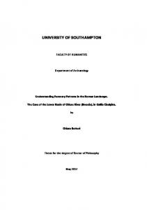
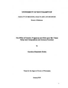
where 1 is an n×1 vector of ones and R is the correlation matrix, the i, j th elements of which are calculated using equation (2.1). The concentrated likelihood is dependent only on the symmetric matrix R and therefore only upon the hyperparameters which are then optimized to maximize the likelihood. This optimization is often referred to as hyperparameter tuning. With the hyperparameters defined, the surrogate model can be used to predict regions which either minimize the model’s prediction of the objective function or maximize its expected improvement (Jones 2001). For more information on the intricacies of kriging the interested reader can consult either Jones et al. (1998) or Forrester et al (2008). It can be observed from the above equations that the calculation of the concentrated likelihood requires the factorization of the correlation matrix, R. If using the Cholesky factorization this can be of order O(n3 ) and, therefore, extremely expensive if the correlation matrix is large. One of the reasons kriging is not typically adopted for design problems with more than 20 variables is the cost of the global optimization necessary to maximize the likelihood. When the number of variables in the problem is large, a large number of sample points are needed to produce an adequate response surface. Jones et al. (1998), for example, advocate the use of 10d initial sample points. Jin et al. (2001) demonstrate that on some test functions, kriging models constructed from 3d sample points can be reasonably accurate. At high dimensions the number of initial design points can be large causing each evaluation of the likelihood to be quite expensive. As the number of dimensions increases so too does the number of hyperparameters requiring optimization and therefore the length of the optimization. As a typical optimization progresses this cost will only increase further as update points are added and the correlation matrix increases in size. Coupling the increasing expense of a single likelihood evaluation with the application of a global optimizer, such as a genetic algorithm, which requires a large number of such evaluations, the total hyperparameter optimization cost can quickly spiral out of control and may even approach that of the high fidelity simulations used in the underlying design problem. Figure 1 helps to demonstrate the cost which can be incurred in optimising the likelihood by demonstrating the increase in time taken to make a single evaluation Article submitted to Royal Society
An Adjoint For Likelihood Maximization
5
Cost of Concentrated Likelihood Evaluation (s)
1 0.9 0.8 0.7 0.6 0.5 0.4 0.3 0.2 0.1 0
0
50
100 150 200 No. of Sample points
250
300
Figure 1. Demonstration of the real time cost of a single evaluation of the concentrated likelihood as the number of sample points increases for an arbitrary 50 variable design problem
as the number of sample points increases for an arbitrary 50 variable problem, the Keane Bump Function taken from Keane & Nair (2005). Assume for example that 300 sample points are included in the initial sampling of the problem, based on this plot a single evaluation of the likelihood will take approximately 1 second on a desktop computer. An optimization of the likelihood which carries out a total of 10,000 evaluations will therefore take approximately 2.8 hours. This represents a significant bottle-neck in the optimization process as a series of these likelihood optimizations, of increasing cost due to the addition of updates, are required throughout the course of a typical kriging based optimization. As well as the local hyperparameter optimization strategies mentioned previously (Park & Baek 2001; Zhang & Leithead 2005; Leithead & Zhang 2007), a number of other strategies have been developed which approach the issue of the cost of hyperparameter tuning from different directions. Initial investigations determined that updating the hyperparameters used to define the krig is extremely important as an optimization progresses. However, it was observed that by optimising the hyperparameters after every other set of updates to the model the total tuning cost could be halved with minimal effect on the efficiency of the optimization (Toal et al. 2008a). Gano et al. (2006) utilised a trust region ratio as a measure of how well a kriging approximation represents the true model. This metric was then used to determine if a model’s hyperparameters required updating. Recently, the authors also demonstrated that the byproduct of a reparameterization of the design problem in order to reduce the total number of variables was a substantial reduction in hyperparameter tuning cost due to a reduction in the size of the correlation matrix (Toal et al. 2008b). The strategies of Toal et al. (2008a, 2008b) , however, involved a substantial global optimization using a genetic algorithm followed by a dynamic hill climber to tune the hyperparameters. In the remainder of this paper we begin to move away from a pure global optimization of the hyperparameters with terminal search towards a hybridized approach by developing an efficient adjoint calculation of the likelihood for use within such a scheme. Article submitted to Royal Society
6
Toal, Forrester, Bressloff, Keane & Holden
3. Traditional Analytical Derivative Calculation The derivation of the analytical gradients of the likelihood with respect to the hyperparameters θl or pl begins by first considering the derivative of the concentrated likelihood, (equation 2.2), ∂φ n ∂σ ˆ2 1 ∂|R| =− 2 − , ∂ψ 2ˆ σ ∂ψ 2|R| ∂ψ
(3.1)
where ψ represents any of the hyperparameters or indeed the regression constant, λ. The derivative of the determinant of a matrix can be expressed in terms of the derivative of the matrix, (Kubota 1994), · ¸ ∂|R| ∂R = |R|Tr R−1 . (3.2) ∂ψ ∂ψ The derivative of the variance with respect to any hyperparameter can be expressed as, · −1 ∂σ ˆ2 1 T ∂R = (y − 1ˆ µ) (y − 1ˆ µ) − ∂ψ n ∂ψ µ ¶T µ ¶¸ ∂µ ˆ ∂µ ˆ T − 1 R−1 (y − 1ˆ µ) − (y − 1ˆ µ) R−1 1 . (3.3) ∂ψ ∂ψ −1
∂µ ˆ However the terms involving ∂ψ are significantly smaller than the ∂R ∂ψ term, and can therefore be neglected. Equation 3.3 can therefore be simplified considerably, (Park & Baek 2001), −1 ∂σ ˆ2 1 T ∂R = (y − 1ˆ µ) (y − 1ˆ µ) . ∂ψ n ∂ψ
(3.4)
The derivative of the inverse of the correlation matrix can be expressed in terms of the derivative of the correlation matrix (Petersen & Pederson 2007), ∂R−1 ∂R −1 = −R−1 R . ∂ψ ∂ψ
(3.5)
Substituting equation 3.5 into equation 3.4 and then into equation 3.1 along with equation 3.2 produces the following expression for the derivative of the concentrated likelihood function with respect to any hyperparameter (Park & Baek 2001), · ¸ · ¸ ∂φ 1 1 T −1 ∂R −1 −1 ∂R = (y − 1ˆ µ ) R R (y − 1ˆ µ ) − Tr R . (3.6) ∂ψ 2ˆ σ2 ∂ψ 2 ∂ψ The derivative of the correlation matrix, R with respect to any hyperparameter is therefore the only remaining unknown and this can be expressed in terms of the derivative of every value within the matrix. Given that the i, j th value of the correlation matrix is given by equation 2.1, the partial derivative with respect to the lth , θ hyperparameter is, ∂Ri,j = −10θl ln 10 ||xil − xjl ||pl Ri,j , ∂θl Article submitted to Royal Society
(3.7)
An Adjoint For Likelihood Maximization
7
and the partial derivative with respect to the lth , p hyperparameter is, ∂Ri,j = −10θl ln ||xil − xjl || ||xil − xjl ||pl Ri,j . ∂pl
(3.8)
The derivatives of the concentrated likelihood function can therefore be calculated using equation 3.6 once the matrices of derivatives of the correlation matrix with respect to each hyperparameter have been defined. In summary, the partial derivatives of the likelihood can be calculated by first calculating the correlation matrix along with the 2d matrices of first derivatives of the correlation matrix, ∂R ∂ψ . The mean, variance and inverse of the correlation matrix can be calculated as normal and then combined to calculate the likelihood as per equation 2.2 and the 2d partial derivatives as per equation 3.6. The calculation of all of the partial derivatives using this method therefore requires the storage of the 2d matrices of first derivatives as well as a number of additional matrix multiplications. The inclusion of a regression constant λ in the correlation matrix (Forrester et al. 2006b) results in a kriging surface which no longer interpolates through the sample points. Adding the regression constant 10λ to the diagonal of the correlation matrix results in the sample points no longer being correlated with themselves. Like the other hyperparameters, θ and p, the regression constant is optimized via maximising the likelihood. Therefore it is important to consider the calculation of the derivative of the likelihood with respect to this constant. As with both θ and p the derivative first requires the calculation of the derivative of the correlation matrix with respect to the hyperparameter of interest. As only the diagonal of the correlation matrix is dependent on the regression constant, the partial derivative of the correlation matrix with respect to the regression constant is itself diagonal in nature, ∂Rii = 10λ ln 10. ∂λ
(3.9)
Using this derivative in conjunction with equation 3.6 will therefore result in the partial derivative of the concentrated likelihood with respect to the regression constant.
4. Introduction to Algorithmic Differentiation Algorithmic differentiation approaches the calculation of derivatives in a slightly different manner to that of traditional analytical differentiation. Here the original computer algorithm used in the calculation of a function is differentiated line by line through application of the chain rule. There are a number of programs which perform this operation automatically given a program’s source code, this is termed automatic differentiation. However, in some circumstances this can lead to an inefficient program as the automatic differentiation process may fail to take account of the structure of the original problem. Mader et al. (2008) for example found that the efficiency of their automatically differentiated computational fluid dynamics solver could be drastically improved after careful consideration of the structure of the underlying problem. Automatically differentiating the entire residual routine resulted in a series of unnecessary computations as the differentiation tool took no account of the sparsity of the flux Jacobian. Article submitted to Royal Society
8
Toal, Forrester, Bressloff, Keane & Holden
There are two modes of algorithmic differentiation, the forward and reverse, or adjoint, mode. Forward mode is akin to traditional differentiation with the differentiated program run once for every input. This produces a partial derivative of every output with respect to a single input each time the program is run. Reverse mode however runs the differentiated program once for every output and therefore obtains all of the partial derivatives of a single output with respect to all inputs for a single run of the differentiated program. The choice of method therefore depends on the nature of the problem. Simplistically, if there are more outputs than inputs it is more efficient to use the forward mode, but if there are more inputs than outputs then it is more efficient to use the reverse mode. The assumption of a pass through the forward differentiated code for every input and a reverse pass for every output is a rather simplistic one. Some automatic differentiation tools can facilitate a vector forward mode which can evaluate multiple partial derivatives in a single pass. Likewise some automatic differentiation tools can facilitate a vector reverse mode whereby the derivatives of multiple outputs can be calculated in a single pass. Both methods save on computation time but incur a memory overhead. To demonstrate the basic process of algorithmic differentiation we consider the simple analytical function y which is dependent on the variables x1 and x2 , µ ¶2 x1 y = sin(x1 x2 ) + . (4.1) x2 Although the partial derivatives of this function can be easily calculated, the simplicity of this function allows the basics of algorithmic differentiation to be demonstrated. The process commences with the definition of the algorithm to calculate the function y. Each line of this algorithm, shown in table 1 using the notation of Griewank (2000), carries out a single operation, i.e. an addition, multiplication, division or trigonometric operation, and terminates in the calculation of y. In this case we begin with the initialisation of the input variables x1 and x2 to v0 and v1 respectively, where vi refers to the ith intermediate variable calculated as the algorithm progresses. The third line multiplies v0 and v1 to give v2 which is equivalent to x1 x2 in equation 4.1, the fourth line calculates xx12 , the fifth, sin(x1 x2 ) and so fourth until the function is calculated. The forward mode of algorithmic differentiation, differentiates each line of this original algorithm in order, resulting in a tangent, (a first derivative vector), of the ith intermediate variable vi , denoted here by v˙ i . For example, the third line of the original algorithm calculated v2 = v0 v1 the tangent of this line is therefore the derivative of v2 with respect to v0 plus the derivative with respect to v1 . Repeating the process through the entire algorithm results in an expression for y˙ which is equivalent to the derivative of the original function with respect to an input, providing appropriate seedings of x˙ 1 and x˙ 2 are defined. These seedings equate to the derivative of each input variable with respect to the required derivative of the overall algorithm. If, for example, the overall derivative of y with respect to x1 is ∂x1 2 required then x˙ 1 = ∂x = 1 and x˙ 2 = ∂x ∂x1 = 0. One can observe from table 1 that 1 ∂y . The forward differentiation given these seedings, y˙ will indeed correspond to ∂x 1 of the original algorithm must therefore be run twice, with the seedings adjusted accordingly, for each input variable. Article submitted to Royal Society
An Adjoint For Likelihood Maximization
9
Table 1. A simple example of forward & reverse algorithmic differentiation original algorithm v0 = x1 v1 = x2 v2 = v0 v1 v3 = vv10 v4 = sin(v2 ) v5 = v32 v6 = v4 + v5 y = v6
forward differentiation v˙ 0 = x˙ 1 v˙ 1 = x˙ 2 v˙ 2 = v˙ 0 v1 + v0 v˙ 1 v˙ 3 = vv˙ 01 − v˙ 1 vv31 v˙ 4 = v˙ 2 cos(v2 ) v˙ 5 = 2v3 v˙ 3 v˙ 6 = v˙ 4 + v˙ 5 y˙ = v˙ 6
reverse differentiation y¯ = 1 v¯6 = y¯ v¯5 = v¯6 v¯4 = v¯6 v¯3 = 2¯ v5 v3 v¯2 = v¯4 cos(v2 ) v¯1 = v¯2 v0 − v¯3 vv13 v¯0 = v¯2 v1 + vv¯13
The reverse, or adjoint mode, proceeds backwards through the original algorithm commencing with the outputs and ending with the inputs. Each line of the reverse algorithm represents the adjoint of the variable defined by the ith line in the original algorithm, with v¯i here denoting the adjoint of the ith variable of the original algorithm. The adjoint of the ith intermediate variable is equivalent to the sum of the partial derivatives of those intermediate variables which are dependant on vi , multiplied by the corresponding adjoint of the dependant intermediate variables. The intermediate variable v6 , for example, affects only y hence the adjoint of v6 is, v¯6 = y¯
∂y = y¯. ∂v6
(4.2)
Likewise, v5 affects only v6 hence v¯5 = v¯6 . Things are complicated somewhat when an intermediate variable in the original algorithm affects a number of the following intermediate variables. Consider, for example, the adjoint of v1 ; as v1 affects both v2 and v3 the adjoint of v1 is the sum of the partial derivatives of v2 and v3 with respect to v1 multiplied by their respective adjoints, v¯1 = v¯2
∂v2 ∂v3 v3 + v¯3 = v¯2 v0 − v¯3 . ∂v1 ∂v1 v1
(4.3)
When this reverse differentiation process is completed and the algorithm run, the resulting values of the adjoints, v¯0 and v¯1 , are equivalent to the partial derivatives, ∂y ∂y ∂x1 and ∂x2 . Unlike the forward mode the reverse mode, presented in table 1, requires only a single run to calculate all of the partial derivatives of y given the initial seeding of y¯, which as there is only one output, equals one. If the original algorithm contained a number of outputs then the reverse mode would be run once for each output with the seeding adjusted in a manner similar to that for the forward mode. A single pass of the reverse mode may, however, be possible if a vector reverse mode is utilised. Even though the above example is very simple, it demonstrates the performance improvements offered when partial derivatives of a single output, as is the case in likelihood maximization, are required. Exactly the same techniques can be applied to any computer algorithm though we now apply them to the calculation of the partial derivatives of the likelihood. Article submitted to Royal Society
10
Toal, Forrester, Bressloff, Keane & Holden
5. Reverse Algorithmic Differentiation of the Likelihood The calculation of the concentrated likelihood, equation 2.2, consists of a single output which is dependent on d pairs of hyperparameters θ and p and a single regression constant, λ, if included. Reverse algorithmic differentiation is therefore the most efficient method to apply to this particular problem, and it is the application of this technique which we now consider. The algorithm to calculate the partial derivatives of the concentrated likelihood via reverse algorithmic differentiation begins with the calculation of the likelihood as normal. This is then followed by a reverse differentiation of the original algorithm which, using information stored during the calculation of the likelihood, calculates all of the partial derivatives. The calculation of the likelihood begins with the construction of the correlation matrix R. This symmetrical matrix is then decomposed using the Cholesky factorization into a lower triangular matrix L where, LLT = R.
(5.1)
This matrix can then be used to calculate the mean, µ ˆ and variance, σ ˆ 2 using equations 2.3 and 2.4 respectively in conjunction with forward and backward substitution. The variance, for example, is calculated through the forward substitution, T1 = L−1 (y − 1ˆ µ) ,
(5.2)
which is followed by the back substitution, T2 = (LT )−1 T1 ,
(5.3)
and finally the vector multiplication, σ ˆ2 =
1 T (y − 1ˆ µ) T2 . n
(5.4)
The vectors T1 and T2 represent two temporary vectors which are necessary for the subsequent calculation of the derivatives. The Cholesky factorization is also used to calculate the natural log of the determinant via, X 1 ln(|R|) = ln Lii . 2 i
(5.5)
With the variance and the log of the determinant known, the concentrated likelihood can be easily calculated using equation 2.2. The reverse mode works backwards beginning from an initial seeding of the adjoint of the likelihood, φ¯ = 1. From this starting point the seeding for the adjoint T¯2 can be calculated to be, (y − 1ˆ µ) T¯2 = − , (5.6) 2ˆ σ2 ∂µ ˆ ¯ 1 using where once again ∂ψ ≈ 0. This seeding can then be used to calculate T¯1 and L ¯ the reversely differentiated back substitution algorithm, where L1 is the adjoint of the upper triangular matrix LT used in the back substitution, equation 5.3. The Article submitted to Royal Society
An Adjoint For Likelihood Maximization
11
¯ 2 , of the lower triangular matrix L used in the forward substitution of adjoint, L equation 5.2 is then calculated using T¯1 and the reversely differentiated forward substitution algorithm. Smith (1995) demonstrated that the adjoint of the log of the determinant of a matrix is equal to the negative of the reciprocal of the diagonal of the lower triangular matrix L resulting from the Cholesky factorization. The ¯ 3 , is therefore, component of the total adjoint due to the log of the determinant, L ¯3 = − 1 . L ii Lii
(5.7)
Hence, the total adjoint for use in Smith’s reversely differentiated Cholesky factorization is, ¯ =L ¯T + L ¯2 + L ¯ 3. L (5.8) 1 When this is then used in conjunction with the original matrix L in Smiths reverse ¯ is calculated. This can then be Cholesky factorisation, the lower triangular matrix R used along with information stored during the original calculation of the correlation matrix to calculate all of the partial derivatives. The derivative of the likelihood with respect to the lth , θ hyperparameter is therefore, X ∂φ ¯ ij = ln 10 −10θl ||xil − xjl ||pl Rij R (5.9) ∂θl ij and the derivative with respect to the lth , p hyperparameter is X ∂φ ¯ ij . −10θl ||xil − xjl ||pl ln ||xil − xjl ||Rij R = ∂pl ij
(5.10)
The derivative of the likelihood with respect to a regression constant λ can be easily ¯ calculated from R, X ∂φ ¯ ii , = 10λ ln 10 R (5.11) ∂λ i assuming that 10λ has been added to the diagonal of the correlation matrix. The algorithms for the Cholesky factorization, forward and backward substitution and their respective reversely differentiated algorithms are presented in the appendix of this paper for the interested reader. Although not an issue in the above formulation, due to the application of the regression term in the construction of the correlation matrix, this matrix may become ill-conditioned when regression is neglected. In such a case the adjoint formulation would not hold, but neither would the initial pass through the algorithm to calculate the likelihood. A small constant regression term could be employed in the construction of the correlation matrix to help prevent ill-conditioning and would have very little impact on the quality of the final kriging model. When a model is constructed through a series of computational experiments exhibiting some form of noise, regression is a necessity and ill-conditioning becomes less of an issue.
6. Computational Efficiency of Derivative Calculations Having described in detail the procedure for calculating the partial derivatives of the likelihood via both the analytical and the reverse algorithmic differentiation Article submitted to Royal Society
12
Toal, Forrester, Bressloff, Keane & Holden
methods, one must now consider each method’s computational efficiency. The analytical method requires the calculation of equation 3.6 for each hyperparameter while the reverse method requires only a single reverse pass of the forward substitution, the backward substitution and the Cholesky factorization to obtain the ¯ which can be used to calculate the partial derivatives via equations 5.9, matrix R 5.10 and 5.11. The question is therefore, by how much does this reduction in the number of calculations improve the performance of the derivative calculation. 4
Relative Cost of Gradient Calculation
3.5
3
2.5
2
Reverse Mode Analytical 1.5
0
5
10
15
20
25 30 No. Variables
35
40
45
50
55
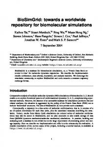
Figure 2. A comparison of the relative costs of calculating all of the partial derivatives of the likelihood via reverse algorithmic differentiation and the analytical formulation
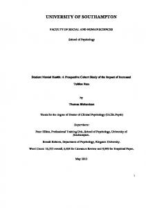
We now consider the relative cost of calculating the likelihood and all derivatives to the cost of calculating only the likelihood. Figure 2 shows the change in this relative cost as the number of dimensions of the underlying problem, to which a kriging surface is fitted, increases. It must be noted that here the number of sample points remains a constant as the number of dimensions increases, 50 points in this case, and that the relative cost includes the calculation of all of the derivatives with respect to θ and p for every dimension as well as the cost of calculating the likelihood itself. The cost obtained for 20 variables therefore equates to the calculation of 40 partial derivatives and the likelihood. By retaining a constant n, Figure 2 shows the effect of purely an increase in problem dimensionality. All of the presented methods were coded and analysed in Matlab. A total of 100 different Latin hypercube sampling plans of the Keane Bump Function, (Keane & Nair 2005), were calculated and stored. Each evaluation of the likelihood and corresponding partial derivatives in Figure 2 were therefore made from a common data set. The likelihood and derivatives of a single set of hyperparameters were evaluated for each of these sample plans. The time for each of these calculations was then recorded and compared to the time taken to calculate of only the likelihood, the resulting relative times were then averaged. The results presented in Figure 2 demonstrate a clear performance advantage when all of the partial derivatives are calculated via the reverse method, with the cost remaining just over half that of the analytical method. The reverse method can also be observed to be less sensitive to an increase in dimensionality with the Article submitted to Royal Society
An Adjoint For Likelihood Maximization
13
relative cost of the reverse method increasing at a slower rate than the analytical method for an increase from five to 50 dimensions. These differences in cost can be explained by analysing the way in which the derivatives are calculated. Consider first the analytical method. In this case the final calculation of a derivative, equation 3.6, requires one additional matrix-matrix multiplication in the calculation of the derivative of the determinant, and three additional matrix-vector multiplications and a vector-vector multiplication in the calculation of the derivative of the variance. Calculating the partial derivative of the likelihood with respect to all of the hyperparameters when fitting a krig to a d dimensional problem therefore requires 2d additional matrix-matrix multiplications, 6d additional matrix-vector multiplications and 2d additional vector-vector multiplications. Including the regression constant increases the expense of calculating all of the derivatives slightly but the cost of calculating this derivative is smaller than for the other hyperparameters due to the sparse nature of the ∂R ∂λ matrix which simplifies the calculations in equation 3.6. The reverse mode however, requires a single reverse pass of the back substitution which is followed by a reverse pass of the forward substitution and then a reverse pass of the Cholesky factorization. Each of these calculations are performed only once and are therefore independent of the number of dimensions in the underlying problem. Only the final step in the derivative calculation, equations 5.9 and 5.10, are dependent on the number of dimensions in the underlying problem, with d calculations of each required. ¯ is lower These final calculations are simplified somewhat by the fact that R ¯ triangular and that the elemental multiplication of the correlation matrix R with R is common to all calculations and can therefore be carried out only once. These final calculations do however require d lower triangular matrices of −10θl ||xil − xjl ||pl and d matrices of ||xil − xjl || to be stored during the initial likelihood calculation. The calculation of a derivative with respect to p is slightly more expensive than calculating a derivative with respect to θ as the natural log of ||xil −xjl || is required.
5
Relative Cost of Gradient Calculation
4.5
Reverse Mode (2d) Reverse Mode (5d) Reverse Mode (10d) Analytical (2d) Analytical (5d) Analytical (10d)
4
3.5
3
2.5
2
1.5 20
25
30
35 No. Variables
40
45
50
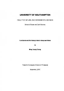
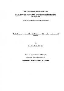
Figure 3. A comparison of effect of sampling density on the relative costs of calculating all of the partial derivatives of the likelihood via reverse algorithmic differentiation and the analytical formulation
Article submitted to Royal Society
14
Toal, Forrester, Bressloff, Keane & Holden
Figure 3 demonstrates how the relative cost of calculating the likelihood and all of the partial derivatives changes as the sampling density of the underlying problem alters. Once again the Keane Bump function is sampled but this time the number of sample points is adjusted according to the number of dimensions in the underlying problem. Sampling densities of 2d, 5d and 10d are all employed. An underlying problem with 25 dimensions will therefore have either 50, 125 or 250 sample points. The results of Figure 3 demonstrate the adjoint method’s relative resistance to an increase in sampling density. The relative cost of the analytical method for example increases by 24.7% when the sample density of the 50 variable problem increases from 2d to 10d whereas the relative cost of the adjoint only increases by 9.3%. These results can be explained by once again analysing the way in which the derivatives are calculated. The number of sample points directly influences the size of the kriging correlation matrix and hence the size of any matrices or vectors used in the subsequent calculations. More importantly this directly affects the cost of the additional matrix-matrix, matrix-vector and vector-vector multiplications required to calculate the likelihood derivatives. As the number of sample points increases so too does the cost of these additional calculations. The problem is compounded at higher dimensions where not only are there more of these calculations, but their cost increases as more sample points are required to produce an accurate response surface. This can be observed in Figure 3 in the divergence of the relative costs of the analytical method as the number of dimensions increases. The calculations carried out by the adjoint method are also affected by the number of sample points and hence size of the correlation matrix. The cost of the reverse forward and backward substitutions and the reverse Cholesky are all dependent on the number of sample points, however unlike the analytical method, these are only carried out once no matter the number of dimensions. Likewise the cost of elemental multiplication of the correlation matrix R with the lower ¯ is dependent on the number of sample points but this is again triangular matrix, R, only carried out once. The calculation of equations 5.9 and 5.10 are dependent on both the number of sample points and the number of dimensions. However, due to the lower triangular nature of the previous elemental multiplication the impact of the number of sample points is reduced somewhat. Combining all of these features produces a method of calculating the partial derivatives of the likelihood which is both more efficient than the analytical method and less prone to large increases in relative cost as sampling density increases. Least squares fitting a quadratic polynomial to the relative costs of the adjoint method, results in an expression for the relative cost with an r2 correlation of 0.993, (−1.43d2 − 2.37s2 + 170d + 237s + 14900) × 10−4 ,
(6.1)
where s denotes the sampling density. Fitting a polynomial to the relative costs of the analytical method results in, (−0.9d2 + 13.7s2 + 36.6ds + 121d − 823s + 32350) × 10−4 ,
(6.2)
giving an r2 correlation of 0.997. The equations of these polynomials reflect the more extensive cross coupling between the number of sample points and the dimensionality of the underlying problem when employing the analytical method. Given a fixed dimensionality the expression for the cost of analytical method also reflects the method’s sensitivity to increasing sampling size. Article submitted to Royal Society
An Adjoint For Likelihood Maximization
15
Table 2. A comparison of the RMS error in the gradients calculated via reverse differentiation and finite differencing to that of the traditional analytical method No. of Variables 2 5 10 15 25
Reverse Differentiation 4.41 × 10⁻¹³ 3.80 × 10⁻¹³ 6.71 × 10⁻¹³ 2.16 × 10⁻¹³ 1.14 × 10⁻¹³
Finite Differencing 2.17 × 10⁻³ 4.95 × 10⁻⁵ 2.00 × 10⁻⁵ 3.42 × 10⁻⁵ 3.94 × 10⁻⁶
The analytical derivative of the likelihood, equation 3.6, assumes a simplified ∂µ ˆ formulation of the derivative of the variance, where the terms due to ∂ψ are ne−1
glected due to the difference in their magnitude relative to the ∂R term. The ∂ψ adjoint formulation presented above also employs this assumption, hence the adjoint of the mean, µ ˆ, and it’s subsequent effect on the initial seeding of the adjoint ¯ is not calculated. An auof the reversely differentiated Cholesky factorisation, L, tomatic differentiation of the likelihood however, may not take into account the relative insignificance of this term and calculate the adjoint of the mean. These additional calculations may result in a less efficient algorithm than the one presented above. Table 2 provides an indication of the numerical accuracy of the gradients obtained via the adjoint method relative to those obtained via the analytical gradient of equation 3.6. Using the test problem of Toal et al. (2008a), a series of DOEs of increasing complexity were created for the purposes of likelihood calculation. The partial derivatives of the likelihood with respect to each of the hyperparameters were then calculated for 50 sets of kriging hyperparameters for each method and compared to those resulting from the analytical method. Table 2 demonstrates such a negligible difference in the magnitude of the results that one could consider the gradients calculated to be almost identical. 20 Reverse Mode Analytical Forward Mode Finite Differencing
18
Relative Cost of Gradient Calculation
16
14
12
10
8
6
4
2
0
5
10
15
20
25 30 No. Variables
35
40
45
50
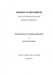
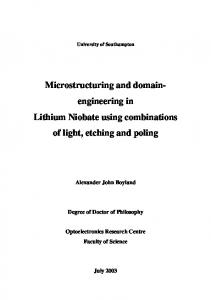
Figure 4. Algorithmic differentiation and the analytical methods compared to finite differencing and forward algorithmic differentiation
Article submitted to Royal Society
16
Toal, Forrester, Bressloff, Keane & Holden
The relative cost of calculating the partial derivatives via the additional methods of finite differencing and a forward algorithmic differentiation are presented in Figure 4. The forward mode results were obtained via a manual forward differentiation of the likelihood calculation. The forward differentiation of the Cholesky factorisation presented in Smith (1995) was employed along with a manually derived forward differentiation of the forward and backward substitutions employed in the calculation of the variance. As with the reverse and analytical formulations, the forward mode takes advantage of the reduction in cost associated with the redundancy of the calculation of µ. ˙ Although the pseudo code of the forward mode is not considered within this paper, this figure serves to reinforce the importance of selecting the appropriate method of algorithmic differentiation for a particular problem. As one can observe, compared to both the analytical and reverse methods, the forward method is more sensitive to an increase in problem dimensionality. Considering that the forward mode requires a pass through the differentiated algorithm for every hyperparameter it is therefore unsurprising that the cost of the derivative calculation becomes an issue. In this case, finite differencing is the most expensive method of calculating the derivatives, requiring two additional full likelihood calculations for every additional variable in the predictive surrogate. Unlike the other methods considered, finite differencing will not produce an exact derivative but rather an approximation to it which is dependent on the step length used, as shown in table 2. The above results indicate that the reverse algorithmic differentiation of the likelihood is the most efficient method of calculating exact partial derivatives. This performance improvement allows for a faster gradient descent search of the likelihood but will also reduce the effort per generation employed in the calculation of gradients when a local search is hybridized with a global search.
7. Conclusions An efficient calculation of the derivatives of the likelihood via an adjoint derived using reverse algorithmic differentiation has been presented. This formulation has been demonstrated to be more efficient than calculating gradients via the traditional analytical method, calculating the likelihood and all of its derivatives for less than twice the cost of a single likelihood evaluation even on a 50 variable problem. The process has also been demonstrated to be less sensitive to an increase in the dimensionality of the problem. Although the reverse algorithmic differentiation process has been applied to a traditional kriging Gaussian kernel, it could be easily extended to other kernels of an alternate formulation or indeed to any other process where a likelihood maximization is required. A similar process could even be applied to the hyperparameter optimization of gradient or Hessian enhanced surrogate models. The adjoint of the likelihood could be employed in a simple local hyperparameter optimization, which may be effective if the sampling density is large, though such an optimization does not guarantee a global optimal set of hyperparameters in a multi-modal likelihood space when the sampling density is small. However it has been proposed that a hybrid global search of the likelihood utilising the adjoint would accelerate hyperparameter optimization considerably. The efficient gradients Article submitted to Royal Society
An Adjoint For Likelihood Maximization
17
provide by the adjoint can be employed in local improvements while global exploration takes place simultaneously. As the derivatives are available more cheaply via the adjoint, the over all tuning cost can be reduced or more extensive global exploration can be carried out for an equivalent total cost. The presented work was undertaken as part of an Airbus funded activity. The authors would like to thank Dr. I. Voutchkov, Dr. A. S´ obester and Mr. G. Endicott of the University of Southampton for their advice and input.
Appendix A. Cholesky factorization, (Smith 1995)
function [ L ] = Cholesky [ R ] % i n i t i a l i z e L as t h e l o w e r t r i a n g l e o f R f or k = 1 : np L(kk) = L(kk) fo r j = k+1:n L(jk) L(jk) = L(kk) end fo r j = k+1:n for i = j : n L(ij) = L(ij) − L(ik)L(jk) end end end Reverse Cholesky factorization, (Smith 1995)
¯ ] = Reverse Cholesky [ L ,L ¯] function [ R ¯ =L ¯ R f or k = n : 1 fo r j = k+1:n for i = j : n ¯ ¯ ¯ R(ik) = R(ik) − R(ij)L(jk) ¯ ¯ ¯ R(jk) = R(jk) − R(ij)L(ik) end end fo r j = k+1:n ¯ ¯ R(jk) = R(jk) L(kk) ¯ ¯ ¯ R(kk) = R(kk) − L(jk)R(jk) end ¯ R(kk) ¯ R(kk) = 2L(kk) end
Article submitted to Royal Society
18
Toal, Forrester, Bressloff, Keane & Holden
Forward Substitution, (Press et al. 1988)
function [ T1 ] = fwardsub [ L , a ] % Where a = (y − 1ˆ µ) a(1) T1 (1) = L(11) f or i = 2 : n S=0 for j = 1 : i − 1 S = S + L(ij)T1 (j) end T1 (i) = a(i)−S L(ii) end
Reverse Differentiation of Forward Substitution
¯ 2 ] = R e v e r s e f w a r d s u b [ T¯1 , L , T1 ] function [ L f or i = n : 2 ¯1 (i) ¯ (i) = TL(ii) a ¯ 2 (ii) = −¯ L a(i)T1 (i) for j = 1 : i − 1 ¯ 2 (ij) = −¯ L a(i)T1 (j) ¯ (i)L(ij) T¯1 (j) = T¯1 (j) − a end end T¯1 (1) ¯ (1) = L(11) a ¯ 2 (11) = −¯ L a(1)T1 (1) Back Substitution, (Press et al. 1988)
function [ T2 ] = bwardsub [ LT , T1 ] (n) T2 (n) = LTT1(nn) f or i = n − 1 : 1 S=0 for j = i + 1 : n S = S + LT (ij)T2 (j) end T2 (i) = TL1 (i)−S T (ii) end
Article submitted to Royal Society
An Adjoint For Likelihood Maximization
19
Reverse Differentiation of Back Substitution
¯ 1 , T¯1 ] = Reverse bwardsub [ T¯2 , LT , T2 ] function [ L f or i = 1 : n − 1 ¯ (i) T¯1 (i) = LTT2 (ii) ¯ 1 (ii) = −T¯1 (i)T2 (i) L fo r j = i + 1 : n ¯ 1 (ij) = −T¯1 (i)T2 (j) L T¯2 (j) = T¯2 (j) − T¯1 (i)LT (ij) end end ¯ (n) T¯1 (n) = LTT2(nn) ¯ 1 (nn) = −T¯1 (n)T2 (n) L
References Broyden, C. 1970 The Convergence of a Class of Double-rank Minimization Algorithms. Journal of the Institute of Mathematics and its Applications 6, 76–90. D’Angelo, S. & Minisci, E. 2005 Multi-Objective Evolutionary Optimization of Subsonic Airfoils by Kriging Approximation and Evolution Control. 2005 IEEE Congress on Evolutionary Computation 2, 1262–1267. Forrester, A. I., Bressloff, N. W. & Keane, A. J. 2006a Optimization Using Surrogate Models and Part Converged Computational Fluid Dynamics Simulations. Proceedings of the Royal Society A 462, 2177–2204. (doi:10.1098/rspa.2006.1679). Forrester, A. I., Bressloff, N. W. & Keane, A. J. 2006b Design and Analysis of “Noisy” Computer Experiments. AIAA Journal 44, 2331–2339. (doi:10.2514/1.20068). Forrester, A. I., S´ obester, A. & Keane, A. J. 2008 Engineering Design via Surrogate Modelling, John Wiley & Sons, Chichester. ISBN 978-0-470-06068-1. Gano, S.E., Renaud, J.E., Martin, J.D. & Simpson, T.W. 2006 Update Strategies for Kriging Models Used in Variable Fidelity Optimization. Structural and Mulitdisciplinary optimization, 32, 287–298. Griewank, A. 2000 Evaluating Derivatives: Principles and Techniques of Algorithmic Differentiation, Society for Industrial and Applied Mathematics Gudla, P. & Ganguli, R. 2005 An Automated Hybrid Genetic-Conjugate Gradient Algorithm for Multimodal Optimization Problems. Applied Mathematics and Computation 167, 1457–1474. Guo, Q., Yu, H. & Xu, A. 2006 A Hybrid PSO-GD Based Intelligent Method for Machine Diagnosis. Digital Signal Processing 16, 402–418. Queipo, N.V., Haftka, R.T., Shyy, W., Goel, T., Vaidyanathan, R., & Tucker, P.K. 2005 Surrogate-Based Analysis and Optimization. Progress in Aerospace Sciences 41, 1–28. Hollingsworth, P., & Mavris, D. 2003 Gaussian Process Meta-Modelling: Comparison of Gaussian Process Training Methods. AIAA 3rd Annual Aviation Technology, Integration and Operations (ATIO) Hoyle, N., Bressloff, N. W. & Keane, A. J. 2006 Design Optimization of a Two-Dimensional Subsonic Engine Air Intake. AIAA Journal 44, 2672–2681. (doi:10.2514/1.16123). Huang, D., Allen, T., Notz, W. & Miller, R. 2006 Sequential Kriging Optimization Using Multiple-Fidelity Evaluations. Structural and Mulitdisciplinary optimization 32, 369– 382. Article submitted to Royal Society
20
Toal, Forrester, Bressloff, Keane & Holden
Jin, R., Chen, W. & Simpson, T. 2001 Comparative Studies of Metamodelling Techniques Under Multiple Modelling Criteria. Structural and Mulitdisciplinary optimization 23, 1–13. Jones, D., Schonlau, A. & Welch, W. 1998 Efficient Global Optimization of Black-Box Functions Journal of Global optimization 13, 455–492. Jones, D. 2001 A Taxonomy of Global Optimization Methods Based on Response Surfaces. Journal of Global optimization 21, 345–383. Keane, A. J. & Nair, P.B. 2005 Computational Approaches for Aerospace Design, John Wiley & Sons, Chichester. ISBN 978-0-470-85540-9. Keane, A. J. 2006 Statistical Improvement Criteria for Use in Mulitobjective Design Optimization. AIAA Journal 44, 879–891. Krige, D.G. 1951 A statistical Approach to Some Basic Mine Valuation Problems on the Witwatersrand. Journal of the Chemical, Metallurgical and Mining Engineering Society of South Africa 52, 119–139. Kubota, K. 1994 Matrix Inversion Algorithms by Means of Automatic Differentiation. Applied Mathematics Letters 7, 19–22. Leithead, W. & Zhang, Y. 2007 O(N 2 )-Operation Approximation of Covariance Matrix Inverse in Gaussian Process Regression Based on Quasi-Newton BFGS Method. Communications in Statistics - Simulation and Computation 36, 367–380. Mader, C., Martins, J., Alonso, J. & van der Weide, E. 2008 ADjoint: An Approach for the Rapid Development of Discrete Adjoint Solvers. AIAA Journal 46, 863–873. (doi:10.2514/1.29123). Martin, J. & Simpson, T. 2005 Use of Kriging Models to Approximate Deterministic Computer Models. AIAA Journal 43, 853–863. Park, J. & Baek, J. 2001 Efficient Computation of Maximum Likelihood Estimators in a Spatial Linear Model with Power Exponential Covariogram. Computers & Geosciences 27, 1–7. Petersen, K. & Perderson, M. 2007 The Matrix Cookbook Press, W., Flannery, B., Teukolsky, S. & Vetterling, W. 1988 Numerical Recipes: The Art of Scientific Computing, Cambridge University Press Sacks, J., Welch, W., Mitchell, T. & Wynn, H. 1989 Design and Analysis of Computer Experiments. Statistical Science 4, 409–435. Sakata, S., Ashida, F., & Zako, M. 2003 Structural Optimization Using Kriging Approximation. Computer Methods in Applied Mechanics and Engineering 192, 923–939. Simpson, T.W., Peplinski, J.D., Koch, P.N., & Allen, J.K. 2001 Metamodels for Computerbased Engineering Design: Survey and Recommendations. Engineering with Computers 17, 129–150. Smith, S.P. 1995 Differentiation of the Cholesky Algorithm. Journal of Computational and Graphical Statistics 4, 134–147. Toal, D. J. J., Bressloff, N. W., & Keane, A. J. 2008a Kriging Hyperparameter Tuning Strategies. AIAA Journal 46, 1240–1252. (doi:10.2514/1.34822). Toal, D. J. J., Bressloff, N. W., & Keane, A. J. 2008b Geometric Filtration Using POD for Aerodynamic Design Optimization. Collection of Technical Papers - 26th AIAA Applied Aerodynamics Conference, Honolulu, HI, United States, 18th − 21st August Wang, G.G., & Shan, S. 2007 Review of Metamodeling Techniques in Support of Engineering Design Optimization. ASME Journal of Mechanical Design 129, 370–380. Zhang, Y., & Leithead, W. 2005 Exploiting Hessian Matrix and Trust-Region Algorithm in Hyperparameter Estimation of Gaussian Process. Applied Mathematics & Computation 171, 1264–1281.
Article submitted to Royal Society