An algebraic algorithm for nonuniformity correction ... - Semantic Scholar
Recommend Documents
The commonly used TPC algorithm is given by (Perry and Dereniak 1993) ..... Hayat MM, Torres SN, Armstrong E, Cain SC, Yasuda B (1999) Statistical ...
Aug 8, 2011 - Optical Engineering 50(8), 087006 (August 2011). Scene-based ... tistical NUC method called the multiscale constant statistics (MSCS). The.
wish to thank Ernest E. Armstrong at the U.S. Air Force Research Laboratory, ... A. F. Milton, F. R. Barone, and M.R. Kruer, âInfluence of nonuniformity on infrared ...
focal plane arrays based on interframe registration. This method ... On the other hand, registration-based NUC ... and f2(x; y), and (u; v) are the Fourier domain coordinates. .... a, while good stability of the algorithm can be achieved with a.
correction algorithm for multichannel remote sensing of coastal waters. This algorithm ... Space Flight Center, U.S. Office of Naval Research, NASA Ocean Biology and Biogeochemistry ..... 2004 and July 7, 2005 over the southern Florida and Bahamas ar
Nov 25, 2011 - phase based on multiplicative correction and on Bootstrap algebraic multigrid. ..... nonlinear GaussâSeidel (BNGS) to the optimality equations (3.4). ...... V. E. Henson, and S. F. McCormick, A Multigrid Tutorial, SIAM, Philadel-.
c 2014 Society for Industrial and Applied Mathematics. Vol. ... methods, the N3 method (nonparametric nonuniform intensity normalization) [14] is popular. ... it is observed in [1] that the parameters used in the past for 1.5 T scanners ...... throug
Filtering Magellan, Palm Bay, Fla., 1993. 19. C. Therrien, Discrete Random Signals and Statistical Signal. Processing Prentice-Hall, Englewood Cliffs, N.J., 1992.
neering, Johns Hopkins University, Baltimore, MD 21218 USA (e-mail: [email protected]; [email protected]). Publisher Item Identifier S ...
email: [email protected]. ABSTRACT. This paper presents a novel procedure for the blind identifi- cation of a linear mixture of Т sources with ¾ sensors.
Jul 21, 2006 - The branch of operations research known as semidefinite programming is relatively new as in- depth study of it has gone on for only about a ...
access channel is to resolve the conflicts that arise when several stations transmit .... The list of queries is said to be (ol, m, n) universal if, for every input I with ]I) ...
Virginia Commonwealth University, VA 23238, USA [email protected]. MICHAEL MANNINO. University of Colorado Denver. Denver, CO 80217, USA.
This paper presents efficient methods for automatic detection and ... sels and optic disc (OD), both of which play important role for ..... On a Pentium-4 PC.
The ULV decomposition (ULVD) is an important member of a class of rank-revealing ... â Department of Computer Science and Engineering, Pennsylvania State ...... sylvania State University, University Park, PA, 2004; available online from ...
descriptions are used to classify future test data for which the class names are unknown. Applications of classification include credit approval, medical diagnosis, store ... This paper introduces a new evolutionary algorithm for classification.
Center, AT&T Bell Laboratories, Room 2D-101, 600 Mountain Avenue,. Murray Hill, NJ 07974, USA. transmission conflict, schedules retransmissions so that,.
10 necessary and sufficient conditions for checking regularity of interval matrices, each of ...... The 2-norm condition number of this matrix is about 4.7 · 108.
By Johannes Buchmann and H. C. Williams*. Abstract. ... of h, it is shown that this technique will produce the value of h in 0(\dp\1+e/(h*R)2) elementary ...
The authors wish to thank Ernest E. Armstrong (OptiMet- rics Inc., USA) for collecting the data, and the United States Air Force Research. Laboratory, Ohio, USA.
where k = 1,..., 4 represent the local numbering of DOFs within each element. ..... (a) Galerkin method. 1/256 1/128 1/64. 1/32 1/16. 10â4. 10â3. 10â2. 10â1. 100.
May 29, 2015 - Recursive Multilevel Solver (pARMS) [29], which consist of ... NA] 29 May 2015 .... For example, in pARMS [29] efficient preconditioners.
An algebraic algorithm for nonuniformity correction ... - Semantic Scholar
We are also grateful to. Ernest Armstrong and the Air Force Research Laboratory, ... R. C. Hardie, K. J. Barnard, J. G. Bognar, and E. A. Watson,. ''High-resolution ...
Ratliff et al.
Vol. 19, No. 9 / September 2002 / J. Opt. Soc. Am. A
1737
An algebraic algorithm for nonuniformity correction in focal-plane arrays Bradley M. Ratliff and Majeed M. Hayat Department of Electrical and Computer Engineering, University of New Mexico, Albuquerque, New Mexico 87131-1356
1. INTRODUCTION Focal-plane array (FPA) sensors are used in many modern imaging and spectral sensing systems. An FPA sensor consists of a mosaic of photodetectors placed at the focal plane of an imaging system. Despite the widespread use and popularity of FPA sensors, their performance is known to be affected by the presence of fixed-pattern noise, which is also known as spatial nonuniformity noise. Spatial nonuniformity occurs primarily because each detector in the FPA has a photoresponse slightly different from that of its neighbors.1 Despite significant advances in FPA and detector technology, spatial nonuniformity continues to be a serious problem, degrading radiometric accuracy, image quality, and temperature resolution. In addition, spatial nonuniformity tends to drift temporally as a result of variations in the sensor’s surroundings. Such drift requires that the nonuniformity be compensated for repeatedly during the course of camera operation. There are two main types of nonuniformity correction (NUC) techniques, namely, calibration-based and scenebased techniques. The most common calibration-based correction is the two-point calibration.2 This method requires that normal imaging system operation be interrupted while the camera images a flat-field calibration target at two distinct known temperatures. The nonuniformity parameters are then solved for in a linear fashion. For IR systems, a blackbody radiation source is typically employed as the calibration target. Calibration must be used when accurate temperature or radiometric measurement is required. However, radiometric accuracy is not needed in some applications. Therefore, a considerable 1084-7529/2002/091737-11$15.00
J. Opt. Soc. Am. A / Vol. 19, No. 9 / September 2002
Ratliff et al.
estimation algorithm. Through use of these motion estimates, a number of gradient-type matrices are computed using pairs of consecutive frames demonstrating pure vertical and pure horizontal subpixel shifts. These matrices are then combined to form an overall correction matrix that is used to compensate for bias nonuniformity across the entire image sequence. The algorithm provides an effective bias correction with relatively few frames. This will be demonstrated with both simulated and real infrared data. Because of its highly localized nature in time and space, the algorithm is easily implemented and computationally efficient, permitting quick computation of the correction matrix that is needed to compensate continually for nonuniformity drift. Another advantage of this algorithm is that it requires only local temporal irradiance variation. Many algorithms (including those that are based on constant-statistics or constant-range assumptions) rely on the assumption that each detector is exposed to a wide range of irradiance levels. Such algorithms typically suffer in performance when a portion of an image sequence lacks sufficient irradiance diversity over time. As demonstrated in this paper, the algebraic technique exhibits considerable robustness to such limitations. This paper is organized as follows. The sensor and motion models are given in Section 2. The algorithm is derived in Section 3, and its performance is studied in Section 4. Finally, the conclusions and future extensions of the proposed technique are given in Section 5.
2. SENSOR AND MOTION MODELS Consider an M ⫻ N image sequence y n generated by a FPA sensor, where n ⫽ 1, 2, 3,... represents the image frame number. A commonly used approximate linear model14 for a FPA-sensor output is given by y n 共 i, j 兲 ⫽ a 共 i, j 兲 z n 共 i, j 兲 ⫹ b 共 i, j 兲 ,
(1)
where z n (i, j) is the irradiance, integrated over the detector’s active area within the frame time, and a(i, j) and b(i, j) are the detector’s gain and bias, respectively. In many sensors, the bias nonuniformity dominates the gain nonuniformity and the latter can be neglected. In this paper we will restrict our attention to such cases and therefore assume that the gain is uniform across all detectors with a common value—without loss of generality—of unity. Thus the observation model becomes y n 共 i, j 兲 ⫽ z n 共 i, j 兲 ⫹ b 共 i, j 兲 .
(2)
It is convenient to associate with each M ⫻ N sensor a bias nonuniformity matrix B defined by
B⫽
冋
b 共 1, 1 兲
b 共 1, 2 兲
b 共 2, 1 兲
b 共 2, 2 兲
]
]
b 共 M, 1兲
b 共 M, 2兲
¯
b 共 1, N 兲
¯
b 共 2, N 兲
¯
b 共 M, N 兲
]
]
册
.
(3)
Moreover, we define I(B) to be the collection of all images that can be generated by a sensor whose bias matrix is B,
according to the model given by Eq. (2). A sensor having a bias matrix B will be referred to as a B-sensor. We also assume that the temperature of the observed objects does not change during the interframe time interval. Thus if two consecutive frames are seen to exhibit strictly horizontal or vertical subpixel global motion, we may then approximate the irradiance at a given pixel in the second frame as a linear interpolation of the irradiance at the pixel and its neighbor from the first frame. This linear interpolation model is selected for its simplicity as an approximation. More precisely, for a pair of consecutive frames exhibiting a purely vertical subpixel shift of ␣ pixels, denoted as an ␣-pair, the kth and the (k ⫹ 1)th frames are related by y k⫹1 共 i ⫹ 1, j 兲 ⫽ ␣ z k 共 i, j 兲 ⫹ 共 1 ⫺ ␣ 兲 z k 共 i ⫹ 1, j 兲 ⫹ b 共 i ⫹ 1, j 兲 ,
0 ⬍ ␣ ⭐ 1.
(4)
Similarly, for a pair of adjacent frames with a purely horizontal subpixel shift of  pixels (denoted as a -pair), we have y m⫹1 共 i, j ⫹ 1 兲 ⫽  z m 共 i, j 兲 ⫹ 共 1 ⫺  兲 z m 共 i, j ⫹ 1 兲 ⫹ b 共 i, j ⫹ 1 兲 ,
0 ⬍  ⭐ 1.
(5)
By convention, a positive ␣ represents downward motion of the scene and a positive  represents rightward motion. In the next section we exploit the relationships given by Eqs. (4) and (5) and use pairs of observed frames to compute algebraically a bias correction map.
3. ALGORITHM DESCRIPTION We begin by discussing the key principle behind the algorithm. The algorithm is based on the ability to exploit shift information between two consecutive image frames exhibiting a purely vertical shift, say, to convert the bias value in a detector element to the bias value of its vertical neighbor. This mechanism will, in turn, allow us to convert the biases of detectors in an entire column to a common bias value. The procedure can then be repeated for every column in the image pair, resulting in an image that suffers from nonuniformity across rows only (i.e., each column has a different, yet uniform, bias value). Now, with an analogous procedure and by using a pair of horizontally shifted images, we can unify the bias values across all rows, which ultimately allows for the unification of all biases in the array to a common value. The details of the algorithm are given next. A. Bias Unification in Adjacent Detectors Suppose that we have two consecutive image frames (frames n and n ⫹ 1, say) for which there is a purely vertical shift ␣ between them. Without loss of generality, consider the output at detectors (1, 1) and (2, 1) of the FPA. According to Eq. (2), y n 共 1, 1 兲 ⫽ z n 共 1, 1 兲 ⫹ b 共 1, 1 兲 ,
(6)
y n 共 2, 1 兲 ⫽ z n 共 2, 1 兲 ⫹ b 共 2, 1 兲 .
(7)
Moreover, we know from the interpolation model of Eq. (4) that
Ratliff et al.
Vol. 19, No. 9 / September 2002 / J. Opt. Soc. Am. A
y n⫹1 共 2, 1 兲 ⫽ ␣ z n 共 1, 1 兲 ⫹ 共 1 ⫺ ␣ 兲 z n 共 2, 1 兲 ⫹ b 共 2, 1 兲 .
B. Vertical and Horizontal Correction Matrices We begin by defining an intermediate vertical correction ˜ with an ␣-pair for a B-sensor as follows: For matrix V B ˜ (1, j) ⫽ 0, and for i ⫽ 2, 3,..., M, dej ⫽ 1, 2,...,N, put V B fine
(8) Now the key step is to form a linear combination of y n (1, 1), y n (2, 1), and y n⫹1 (2, 1) so that the irradiance values are canceled and only the biases remain. More precisely, we form ˜ B共 2, 1 兲 ⫽ V
1
␣
˜ 共 i, j 兲 ⫽ V B 关 ␣ y n 共 1, 1 兲 ⫹ 共 1 ⫺ ␣ 兲 y n 共 2, 1 兲
(9)
␣
(12)
Hence
¯
0
0
b 共 1, 1 兲 ⫺ b 共 2, 1 兲
b 共 1, 2 兲 ⫺ b 共 2, 2 兲
b 共 2, 1 兲 ⫺ b 共 3, 1 兲
b 共 2, 2 兲 ⫺ b 共 3, 2 兲
]
] b 共 M ⫺ 1, 2 兲 ⫺ b 共 M, 2兲
use of Eqs. (6), (7), and (8), reduces to (10)
˜ (2, 1) is added to y (2, 1), we obtain Now if V B n
0
¯
b 共 M, 1, 1 兲 ⫺ b 共 M, 1兲
˜ B共 2, 1 兲 ⫽ b 共 1, 1 兲 ⫺ b 共 2, 1 兲 . V
关 ␣ y n 共 i ⫺ 1, j 兲 ⫹ 共 1 ⫺ ␣ 兲 y n 共 i, j 兲
⫽ b 共 i ⫺ 1, j 兲 ⫺ b 共 i, j 兲 .
˜ B later) which, upon (we will formally define the matrix V
冋
1
⫺ y n⫹1 共 i, j 兲兴
⫺ y n⫹1 共 2, 1 兲兴 ,
˜B ⫽ V
1739
b 共 1, N 兲 ⫺ b 共 2, N 兲
¯
b 共 2, N 兲 ⫺ b 共 3, N 兲
¯
b 共 M ⫺ 1, 冣 ⫺ b 共 M, N 兲
]
]
册
.
(13)
Now the vertical correction matrix VB is calculated by performing a partial cumulative sum down each column ˜ . of V More precisely, for i ⫽ 2, 3,..., M and j B ⫽ 1, 2,...,N, we define i
˜ B共 2, 1 兲 ⫽ z n 共 2, 1 兲 ⫹ b 共 1, 1 兲 . y n 共 2, 1 兲 ⫹ V
(11)
Hence the bias of the (2, 1)th detector element b(2, 1) is converted to b(1, 1).
VB ⫽
冋
VB共 i, j 兲 ⫽
兺 V˜ 共 r, j 兲 ⫽ b 共 1, j 兲 ⫺ b 共 i, j 兲 ,
so that
¯
0
0
b 共 1, 1 兲 ⫺ b 共 2, 1 兲
b 共 1, 2 兲 ⫺ b 共 2, 2 兲
b 共 1, 1 兲 ⫺ b 共 3, 1 兲
b 共 1, 2 兲 ⫺ b 共 3, 2 兲
]
]
b 共 1, 1 兲 ⫺ b 共 M, 1兲
b 共 1, 2 兲 ⫺ b 共 M, 2兲
0
¯
b 共 1, N 兲 ⫺ b 共 2, N 兲
¯
b 共 1, N 兲 ⫺ b 共 3, N 兲
¯
b 共 1, N 兲 ⫺ b 共 M, N 兲
¯
z k 共 1, N 兲 ⫹ b 共 1, N 兲
]
]
册
Observe now that if VB is added to an arbitrary raw frame y k from I(B),then
y k ⫹ VB ⫽
冋
z k 共 1, 1 兲 ⫹ b 共 1, 1 兲
z k 共 1, 2 兲 ⫹ b 共 1, 2 兲
z k 共 2, 1 兲 ⫹ b 共 1, 1 兲
z k 共 2, 2 兲 ⫹ b 共 1, 2 兲
]
]
z k 共 M, 1兲 ⫹ b 共 1, 1 兲
z k 共 M, 2兲 ⫹ b 共 1, 2 兲
This same procedure may now be applied to the bias˜ (2, 1)] and adjusted (2, 1)th pixel [that is, y n (2, 1) ⫹ V B the original (3, 1)th pixel effectively to convert the bias of the (3, 1)th detector from b(3, 1) to b(1, 1). This procedure may be applied down the entire column, effectively unifying all biases of the column to b(1, 1). Clearly we can repeat the same procedure for other columns with the same ␣-pair. Moreover, an analogous procedure can be performed across all rows with a -pair. The general algorithm will be discussed next.
(14)
B
r⫽2
¯
z k 共 2, N 兲 ⫹ b 共 1, N 兲
¯
z k 共 M, N 兲 ⫹ b 共 1, N 兲
]
]
册
.
(15)
.
(16)
Indeed, in the vertically corrected frame of Eq. (16), the bias values down each column have effectively been unified to the bias value of the topmost pixel (the columnbias ‘‘leader’’). Now if we define the column-corrected sensor bias matrix B⬘ ⫽
冋
b 共 1, 1 兲
b 共 1, 2 兲
]
]
b 共 1, 1 兲
b 共 1, 2 兲
¯ ]
¯
b 共 1, N 兲 ] b 共 1, N 兲
册
,
(17)
1740
J. Opt. Soc. Am. A / Vol. 19, No. 9 / September 2002
Ratliff et al.
then we can identify y k ⫹ VB as a member of I(B⬘ ). More compactly, we maintain that VB ⫹ I(B) ⫽ I(B⬘ ). Clearly a similar procedure can be followed with a -pair to obtain a horizontal correction matrix HB , which, when added to any raw image, will unify the bias values across each row. More precisely, for i ⫽ 1, 2,...,M and j ˜ (i,1) ⫽ 0, and ⫽ 2, 3,...,N, put H ˜ 共 i, j 兲 ⫽ H
1

关  y m 共 i, j ⫺ 1 兲 ⫹ 共 1 ⫺  兲 y m 共 i, j 兲
⫺ y m⫹i 共 i, j 兲兴 .
(18)
HB is then computed by performing a partial cumulative ˜ (i, j). Thus the resulting horisum across each row of H ˜ B becomes zontal correction matrix H
HB ⫽
冋
¯
0
b 共 1, 1 兲 ⫺ b 共 1, 2 兲
b 共 1, 1 兲 ⫺ b 共 1, 3 兲
0
b 共 2, 1 兲 ⫺ b 共 2, 2 兲
b 共 2, 1 兲 ⫺ b 共 2, 3 兲
]
]
]
0
b 共 M, 1兲 ⫺ b 共 M, 2兲
b 共 M, 1兲 ⫺ b 共 M, 3兲
¯
b 共 M, 1兲 ⫺ b 共 M, N 兲
]
0
b 共 1, 1 兲 ⫺ b 共 1, 2 兲
b 共 1, 1 兲 ⫺ b 共 1, 3 兲
0
b 共 1, 1 兲 ⫺ b 共 1, 2 兲
b 共 1, 1 兲 ⫺ b 共 1, 3 兲
]
]
]
0
b 共 1, 1 兲 ⫺ b 共 1, 2 兲
b 共 1, 1 兲 ⫺ b 共 1, 3 兲
and indeed
C ⫽ VB ⫹ HB⬘ ⫽
冋
b 共 1, 1 兲 ⫺ b 共 1, N 兲 b 共 2, 1 兲 ⫺ b 共 2, N 兲
C. Total Correction Matrix The principle of total correction is now clear. First, for any raw ␣-pair obtained from a B-sensor, compute a vertical correction matrix VB . Next, add VB to a -pair from the B-sensor. [Recall that adding VB to any raw frame results in an image in I(B⬘ ) as if it were obtained from the vertically corrected B⬘ -sensor, where B⬘ is defined in Eq. (17).] Next, use the vertically corrected -pair, denoted as a  ⬘ -pair, to compute the horizontal correction matrix HB⬘ . The total correction matrix C is then formed by adding HB⬘ to VB . A straightforward calculation shows that
冋
⬘
¯
Next we use the ability to unify the bias values across columns or rows to unify the biases of the entire array to a common value.
HB⬘ ⫽
collectively introduce error (or noise) in the bias correction matrix. To reduce the effect of this noise, we first obtain two collections C␣ and C which consist of many distinct ␣- and -pairs, respectively. With these collections, we can compute many vertical and horizontal correction matrices and form averaged vertical and horizontal cor¯ B and H ¯ B , respectively. rection matrices, denoted V ⬘ Moreover, we observe from Eq. (20) that all rows of HB⬘ are ideally identical; therefore a second average can be ¯ B , resulting in a horiperformed down each column of H ⬘ ᠬ B . This vector can then be replizontal row vector H ⬘ cated M times to form the M ⫻ N averaged horizontal ញ B . Thus in practice, it is these V ¯B correction matrix H ⬘ ញ and HB that are summed to generate the final correction
¯
]
(19)
D. Shift Estimation The collections of image pairs C␣ and C are generated through the use of the gradient-based shift-estimation algorithm described by Irani and Peleg15 and Hardie et al.16 The gradient-based shift estimator first estimates the gradient at each point in one image by use of a Prewitt operator. With a first-order Taylor series approximation, it is possible to predict the values of a second frame (assumed to be a shifted version of the first) based on the first frame, the gradient from the first frame, and the shift between the frames. In our application, we have
¯
b 共 1, 1 兲 ⫺ b 共 1, N 兲
¯
b 共 1, 1 兲 ⫺ b 共 1, N 兲
]
册
,
0
b 共 1, 1 兲 ⫺ b 共 1, 2 兲
b 共 1, 1 兲 ⫺ b 共 1, 3 兲
b 共 1, 1 兲 ⫺ b 共 2, 1 兲
b 共 1, 1 兲 ⫺ b 共 2, 2 兲
b 共 1, 1 兲 ⫺ b 共 2, 3 兲
]
]
]
b 共 1, 1 兲 ⫺ b 共 M, 1兲
b 共 1, 1 兲 ⫺ b 共 M, 2兲
b 共 1, 1 兲 ⫺ b 共 M, 3兲
which is the desired total correction matrix. Notice that when C is added to any raw image frame in I(B), all bias values become b(1, 1), as desired. In practice, it is observed that there is error associated with the linear interpolation approximation of Eqs. (4) and (5) and error in estimating the shifts ␣ and , which
.
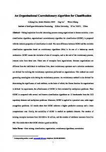
matrix C. As will be shown in Section 4, relatively few frame pairs from each collection are needed to compute an effective correction matrix. A block diagram of the presented NUC algorithm is shown in Fig. 1.
b 共 1, 1 兲 ⫺ b 共 1, N 兲
册
(20)
¯
b 共 1, 1 兲 ⫺ b 共 1, N 兲
¯
b 共 1, 1 兲 ⫺ b 共 2, N 兲
¯
b 共 1, 1 兲 ⫺ b 共 M, N 兲
]
册
,
(21)
knowledge of the two frames and we are able to estimate the gradient. What we do not know is the shift between the frames. The shifts are estimated through a leastsquares technique that minimizes the error between the observed second frame and the predicted second frame. While the gradient-based technique has been shown to
Ratliff et al.
Vol. 19, No. 9 / September 2002 / J. Opt. Soc. Am. A
Fig. 1.
1741
Block diagram of the proposed NUC algorithm.
yield reliable estimates, Armstrong et al.17 found that the accuracy of the shift estimates is compromised by the presence of spatial nonuniformity. This estimation error can be minimized by first smoothing the original image sequence with an R ⫻ R mask, which effectively reduces the nonuniformity. Through this prefiltering of the image sequence, shift estimate accuracy is improved significantly. The resulting shift estimates are then analyzed for acceptable shifts. Acceptable subpixel shifts are defined as those in the interval [⫺1, 1] for both pure horizontal and pure vertical motion. Moreover, we define a tolerance parameter ⑀, which is used to define the maximum allowable deviation from the ideal zero shift in a direction orthogonal to the dominant motion direction. Other computationally efficient registration techniques are available that are shown to perform well in the presence of fixed-pattern noise18 and may be used in place of the gradient-based algorithm. It is also possible that we can substitute controlled motion (i.e., induced motion such that the shifts are known), thereby obviating the need for a motion-estimation algorithm. E. Further Remarks Algorithm robustness is improved by considering three important issues: (1) selection of the starting collection (i.e., C␣ or C ), (2) treatment of frame pairs with positive and negative shifts, and (3) sensitivity to the tolerance parameter ⑀. Once shift estimation is completed, the best starting collection must be determined. This decision is made simply by selecting the collection with the highest number of pairs of frames. Such a selection is made because most of the spatial nonuniformity is encountered when the first averaged correction matrix is computed. With use of the larger collection, error in the bias estimates is reduced as more correction matrices are averaged. Each pair of frames in collections C␣ and C may exhibit a respective shift that is either positive or negative. When each correction matrix is computed, the shift polarity determines the starting row or column. As an example, if an M ⫻ N frame pair having a positive horizontal shift is used—with our shift sign convention—the algorithm starts in column 1 and computes the bias estimates in a rightward direction. If the frame pair exhibits a negative horizontal shift, the algorithm instead begins with column N and computes the bias estimates in a leftward direction. The vertical motion cases are analogous. By considering each of these cases, the algorithm can find and use more frame pairs in accordance with the shift direction.
Finally, for all data tested, we learned that sufficient frame pairs were found when parameter ⑀ was given a value of 0.05 pixels. As higher values of ⑀ are allowed, no major decrease in the visual quality of the corrected images is observed until this parameter approaches 0.2 pixel, beyond which striping artifacts across rows or columns will begin to appear.
4. PERFORMANCE ANALYSIS A. Accuracy of Shift Estimation A study was performed on the accuracy of the gradientbased shift-estimation technique used in this paper. In general, the shift-estimation algorithm, in the presence of little or no spatial nonuniformity, demonstrates a high level of accuracy. However, the accuracy of shift estimation suffers as the amount of nonuniformity increases. To observe this effect, the average absolute error in the shift estimates was calculated as a function of bias nonuniformity standard deviation for a typical 8-bit, 128 ⫻ 128, 200-frame image sequence. The result is shown in Fig. 2. A zero-mean Gaussian model was used to independently generate the simulated bias nonuniformities. It is seen that the error in shift estimation increases sharply as the level of nonuniformity increases beyond a certain cutoff in signal-to-noise ratio, which depends on the spatial-frequency content of the true scene sequence. In the example considered, this cutoff occurred at a bias nonuniformity standard deviation of 5 (based on an 8-bit gray scale).
Fig. 2. Average absolute error in the shift estimates as a function of the standard deviation of the bias nonuniformity for a 200-frame sequence. A true shift of 0.5 pixel was used in the simulations.
1742
J. Opt. Soc. Am. A / Vol. 19, No. 9 / September 2002
Application of a smoothing filter to the raw images before shift estimation greatly reduced the shift error, since the spatial nonuniformity was considerably reduced as a result of smoothing. In practice the best mask size will depend on the strength of the nonuniformity and the spatial-frequency content of the scene. A surface plot is displayed in Fig. 3 that shows the average absolute error in the shift estimates as a function of the standard deviation of bias nonuniformity and the mask size. As seen from the plot, the shift error can be reduced significantly if a sufficiently large smoothing filter is employed, even for severe nonuniformity cases, as long as the smoothed images maintain sufficient spatial diversity to allow shift estimation. B. Nonuniformity Correction with Simulated Data A sequence of clean images (in the visible-light range) was used to generate two types of simulated image sequences with bias nonuniformity. The first type consisted of sequences for which subpixel motion was simulated by using linear interpolation, which is fully compatible with our algorithm. As expected when this type of simulated data was used in the algorithm along with the true shift values, perfect NUC was achieved with only four image frames (one ␣-pair and one -pair). The second type of image sequence consists of a more realistic nonlinear shift mechanism. Global motion is generated by first shifting a high-resolution image (e.g., a 1280 ⫻ 1280 image) by multiples of a whole pixel and then down-sampling the shifted image back to the 128 ⫻ 128 grid by means of pixel averaging. This shift mechanism simulates the practical situation when the true object (i.e., the high-resolution image) is moving and each detector in the FPA generates a voltage proportional to the total irradiance collected by its active area. Through this down-sampling technique we can generate subpixel shifts between image frames that are as small as the down-sampling ratio (i.e., 0.1 pixel in this case). All image sequences created were down-sampled by factors ranging from 2 to 10. As a result of down-sampling, the produced sequences were aliased. Clearly as the amount of aliasing increases, the accuracy of our linearinterpolation approximation [given in Eqs. (4) and (5)] decreases, in which case we would expect to see degradation in the NUC capability. A 300-frame, 128 ⫻ 128, 8-bit aliased image sequence (down-sampled by a factor of 4) was generated with 0.5pixel shifts. The sequence originally contained 150 ␣-pairs and 149 -pairs. Zero-mean Gaussian noise with standard deviation of 20 was added to each frame of the image sequence to bring about bias nonuniformity. The sequence was then blurred with a 10 ⫻ 10 smoothing mask before shift estimation. We obtained and used 144 acceptable ␣-pairs and 138 acceptable -pairs. Figures 4(a) and 4(b) show frame 1 from the image sequence before and after addition of the simulated bias nonuniformity, respectively. Figure 4(c) shows frame 1 from the image sequence after correction with our algorithm. Despite the presence of aliasing, very good NUC is achieved. 1. Effect of Lack of Temporal Scene Diversity The simulated sequence was also designed to show another advantage of the algebraic technique. The se-
Ratliff et al.
quence had the property that detectors in the top part of the image were exposed to high values (i.e., the sky in the visible-light range) while the detectors in the bottom portion of the image were exposed to low irradiance (i.e., buildings and trees). The simulated motion allowed only the detectors in the middle portion of the sequence to have the benefit of temporal scene diversity as a result of being exposed to both low and high scene values. To determine the effect of this lack of scene diversity on statistical scene-based algorithms, we subjected the simulated frames to the (bias-only version) constant-statistics algorithm of Harris and Chiang.6 The corrected image frame 1 is shown in Fig. 4(d). As can be seen, this technique has difficulty with regions where irradiance diversity is not present (i.e., in the top and bottom portions of the image). In contrast, the algebraic algorithm does not suffer from such conditions. This is so provided that sceneirradiance does not significantly change (i.e., the temperature of objects within the scene does not vary greatly) between adjacent image frames, as the algorithm would be sensitive to such conditions. However, it is important to note that because we are using the shift-estimation algorithm, two adjacent image frames must present some scene diversity in order for the algorithm to detect and accurately estimate the motion. In cases where motion is known a priori (through precisely controlled motion), such scene diversity is not required. 2. Dependence of Performance on Image Sequence Length A study was performed to determine the number of frame pairs required to generate accurate estimates of the bias nonuniformity. The simulated sequence consisted of 500 frames of 128 ⫻ 128, 8-bit images, and the biasnonuniformity standard deviation was selected as 20. The dependence of the average absolute error (overall pixels) on the number of frame pairs used for correction is depicted in Fig. 5. We observe that in the example considered, the average absolute error in the bias estimation reduces to a very low constant level (approximately 1.25%) after approximately 100 frames. We suspect that this limiting value is primarily attributed to shiftestimation error, which does not vanish, as expected, with an increase in the number of frames used by the NUC algorithm.
Fig. 3. Average absolute error in the shift estimates as a function of bias nonuniformity standard deviation and the size R of the smoothing mask.
Ratliff et al.
Vol. 19, No. 9 / September 2002 / J. Opt. Soc. Am. A
1743
Fig. 4. (a) Frame 1 from the down-sampled image sequence before addition of bias nonuniformity, (b) frame 1 from the down-sampled image sequence after the addition of bias nonuniformity, (c) frame 1 from the image sequence corrected by use of the algebraic NUC algorithm, (d) frame 1 from the image sequence corrected by use of Harris’s (bias-only version) constant-statistics NUC technique.
3. Sensitivity to Error in Shift Estimation We now examine the sensitivity of algorithm performance to error in the shift estimates. We used a simulated 8-bit, 200-frame, aliased image sequence, similar to the sequence of Fig. 4, where the true shift values in the pure horizontal and pure vertical motion were 0.5 pixel. With the true shifts known, the algorithm was deliberately supplied with inaccurate shifts and the resulting average absolute bias-estimate error was computed for different levels of bias nonuniformity, as shown in Fig. 6. We may first observe that when ideal shifts of 0.5 are used, the bias estimate error is approximately zero, regardless of the nonuniformity level. However, for incorrectly assumed shifts beyond 0.5, we notice an almost linear increase in the bias-estimate error. The more interesting case occurs when the incorrectly assumed shift values are below 0.5. In this case, the shift error increases progressively with the incorrect shift. This behavior is ex-
Fig. 5. Average absolute error in the estimation of bias nonuniformity as a function of the number of frame pairs used in generating the correction matrix. In this example, the bias nonuniformity has a zero mean and a standard deviation of 20.
1744
J. Opt. Soc. Am. A / Vol. 19, No. 9 / September 2002
plained by examining the role of the ␣ and  shift parameters in Eqs. (12) and (18). Computing the entries of the correction matrix involves a division by the appropriate presumably correct shift value, forcing the calculation of the correction matrix to be particularly sensitive to small values (and the corresponding fluctuations) of the assumed shift. This adverse effect will be re-examined and reduced when we consider real infrared imagery in subsection 4.C. We also observe that bias-estimation error is insensitive to the level of bias nonuniformity regardless of the error in the assumed shift estimates. However, we need to be cautious in interpreting this result, bias nonuniformity does affect the accuracy of shift estimation (as was shown in Fig. 3). In generating the graph in Fig. 6, however, we exercised full control over the error in the assumed shift. In general, our results show that the combined effect of nonuniformity and shift-estimation error begins to severely degrade the visual quality of the corrected images when the relative error in the shift estimates is in excess of approximately 20%. Thus we conclude that accurate knowledge of the shift is critical for the operation of our NUC algorithm. 4. Effect of Gain Nonuniformity We now examine the algorithm’s performance in the presence of gain nonuniformity in addition to bias nonuniformity. Gain nonuniformity was simulated by using Gaussian random noise with a mean of 1 and varying standard deviation. An 8-bit, 100-frame, aliased (down sampled by a factor of 10:1) image sequence, similar to the sequences previously considered, was processed with our algorithm. Figure 7 shows the error in the calculated bias values as a function of the standard deviations of the bias and gain nonuniformities under the assumption that true shifts are used. We also repeated the calculations using estimated shift values, as shown in Fig. 8. A 10 ⫻ 10 smoothing mask was employed before the shift estimation process. The two plots show similar behavior, namely, that as the severity of the gain nonuniformity increases, so does the error in the bias estimates. When true shifts are used, the role of bias nonuniformity on the performance, unlike the level of gain nonuniformity, becomes irrelevant. On the other hand, when the shifts are estimated, both types of nonuniformity contribute to the error. This is expected since we have observed earlier that the shift estimates are degraded as a result of the bias nonuniformity. Overall, we observe that gain nonuniformity can have a harmful effect on the accuracy of the bias estimates. Though the accuracy of the bias estimates is affected, it is important to note that the visual quality of the corrected image sequences is still good. This is so because the algorithm effectively incorporates the gain nonuniformity into the bias correction map and therefore removes much of it. It is important to note that in all cases where ideal shift values were used, the nonuniformity pattern was always removed after correction. In the case where shift estimates were used, striping artifacts appeared in the corrected sequence whenever the nonuniformity was severe. These artifacts arise mainly as a result of significant error in the shift estimates.
Ratliff et al.
Fig. 6. Average absolute error of the bias estimates as a function of bias nonuniformity standard deviation and shift value.
Fig. 7. Average absolute error in the computed bias values as a function of the standard deviations of gain and bias. The correction algorithm incorporated the true shift values.
Fig. 8. Average absolute error in the computed bias values as a function of the standard deviations of gain and bias. The correction algorithm incorporated the estimated shift values.
C. Nonuniformity Correction with Real Infrared Data The proposed algorithm was tested with real infrared image sequences. The data sets were collected using an 8-bit, 128 ⫻ 128-array, InSb FPA camera (Amber Model AE-4128) operating in the 3–5-m range (the data were generated at the Air Force Research Laboratory, Dayton, Ohio). For all IR data, a 3 ⫻ 3 mask was used to smooth the images before shift estimation. Using two sets of real infrared data sequences, we found that 50–75 frame pairs
Ratliff et al.
in the first direction and 10–20 frame pairs in the second direction were sufficient to produce an effective correction matrix. In the first data set, which consisted of 500 frames, there were 139 ␣-pairs and 47 -pairs when a value of 0.05 was employed for the shift tolerance parameter ⑀. Figure 9(a) displays frame 1 from the 500-frame infrared image sequence. Frame 1 of the infrared image sequence after correction by Harris’s algorithm is shown in Fig. 9(b) and is compared with correction by the algebraic technique, which is shown in Fig. 9(c). The corrected image obtained from the algebraic algorithm contains undesirable striping artifacts, which are due mainly to inaccurate shift estimates, and can be understood in the context of Fig. 6. When inaccurate shifts with values close to zero are used, error in the bias estimates is known to increase dramatically, as discussed earlier in Subsection 4.B. The striping problem can be largely overcome by limiting the acceptable shift range to shifts that are in the interval [0.5, 1.0]. The result for this limited shift range is
Vol. 19, No. 9 / September 2002 / J. Opt. Soc. Am. A
1745
shown in Fig. 9(d); the striping has effectively disappeared. It is interesting to note that the use of the restricted shifts resulted in only 49 ␣-pairs and 18 -pairs; this excluded many of the problematic shift estimates. Again, these problematic shifts are those that contained significant error and had a value close to zero. For comparison, the matrices (scaled to 256 dynamic levels) for the correction of Figs. 9(c) and 9(d) are displayed in Figs. 10(a) and 10(b), respectively. In the first correction map, the undesirable striping effects are clearly visible; however, in the second one the artifacts are not noticeable. Examples from a second 8-bit, 400-frame real infrared image sequence, collected 4 h later by the same camera, are shown in Figs. 11(a) and 11(b). Figure 11(c) displays the correction made with Harris’s algorithm. In this example, which also used the same shift-tolerance parameter ( ⑀ ⫽ 0.05) and restricted shifts (shifts in the interval [0.5, 1]), 43 ␣-pairs and 11 -pairs were found and used by the algorithm.
Fig. 9. (a) Frame 1 from infrared data set 1, (b) correction by Harris’s method, (c) correction by the algebraic algorithm (unrestricted shifts), (d) correction by the algebraic technique with the shifts restricted to the interval [0.5, 1.0].
1746
J. Opt. Soc. Am. A / Vol. 19, No. 9 / September 2002
Ratliff et al.
Fig. 10. (a) Nonuniformity correction map associated with the image of Fig. 9(c), (b) nonuniformity correction map associated with the image of Fig. 9(d).
Fig. 11. (a) Frame 100 from infrared data set 2, (b) correction by the algebraic technique (restricted shifts), (c) correction by Harris’s constant-statistics algorithm.
Ratliff et al.
5. CONCLUSIONS We have developed an algebraic scene-based technique for correction of bias nonuniformity in focal-plane arrays. The performance of the algorithm was thoroughly studied through the use of both simulated and real infrared data. The strength of the proposed algorithm is in its simple algebraic nature. Because of this, the algorithm is computationally efficient and easily implemented. It is shown that an effective correction map can be obtained quickly with use of relatively few image frames. Also, the algorithm’s performance has shown robustness to lack of scene-irradiance diversity, thus demonstrating its advantage over some statistical scene-based techniques. We showed that accurate motion estimation is crucial for acceptable nonuniformity correction, and that the gradient-based, shift-estimation algorithm employed produced reliable shift estimates. We also showed that our algorithm is most sensitive to error in small shift values. This adverse effect was largely overcome by restricting the acceptable subpixel shift range to shifts in excess of 0.5 pixel, which drastically improved bias estimation while reducing the number of frame pairs used for correction. We also showed that significant gain nonuniformity can have a severe effect on the accuracy of the bias estimates, though good visual correction is still possible in the presence of gain nonuniformity. In principle, generalization of the algorithm to incorporate two-directional shifts is possible at the expense of substantial added complexity. A promising course that we are currently undertaking is to use our algorithm in conjunction with absolute calibration to achieve radiometrically accurate nonuniformity correction. Our expectation is that if absolute blackbody calibration is performed on only a fraction of the array elements without halting the function of remaining array elements, then the algorithm can be used to transfer the calibration from the calibrated detectors to the remaining uncalibrated detectors. In this way, we achieve radiometrically accurate correction without halting the operation of the camera during the course of the calibration process. Clearly, the algebraic (nonstatistical) nature of the algorithm is key to linking scene-based and calibration-based techniques without compromising radiometric accuracy. The performance analysis carried out in this paper can be useful in setting a guideline for the expected degree of radiometric accuracy.
Vol. 19, No. 9 / September 2002 / J. Opt. Soc. Am. A
REFERENCES 1. 2. 3.
4. 5.
6.
7.
8.
9.
10.
11. 12.
13.
14. 15.
ACKNOWLEDGMENTS This research was supported by the National Science Foundation Faculty Early Career Development (CAREER) Program MIP-9733308. We are grateful to J. Scott Tyo for many valuable discussions regarding the possibility of integrating calibration-based techniques with the reported algorithm. We are also grateful to Ernest Armstrong and the Air Force Research Laboratory, Dayton, Ohio, for providing us with IR imagery. M. Hayat’s e-mail address is [email protected].
1747
16.
17.
18.
A. F. Milton, F. R. Barone, and M. R. Kruer, ‘‘Influence of nonuniformity on infrared focal plane array performance,’’ Opt. Eng. 24, 855–862 (1985). D. L. Perry and E. L. Dereniak, ‘‘Linear theory of nonuniformity correction in infrared staring sensors,’’ Opt. Eng. 32, 1853–1859 (1993). P. M. Narendra and N. A. Foss, ‘‘Shutterless fixed pattern noise correction for infrared imaging arrays,’’ in Technical Issues in Focal Plane Development, W. S. Chan and E. Krikorian, eds., Proc. SPIE 282, 44–51 (1981). P. M. Narendra, ‘‘Reference-free nonuniformity compensation for IR imaging arrays,’’ in Smart Sensors II, D. F. Barbe, ed., Proc. SPIE 252, 10–17 (1980). J. G. Harris, ‘‘Continuous-time calibration of VLSI sensors for gain and offset variations,’’ in Smart Focal Plane Arrays and Focal Plane Array Testing, M. Wigdor and M. A. Massie, eds., Proc. SPIE 2474, 23–33 (1995). J. G. Harris and Y. M. Chiang, ‘‘Nonuniformity correction using constant average statistics constraint: Analog and digital implementations,’’ in Infrared Technology and Applications XXIII, B. F. Andersen and M. Strojnik, eds., Proc. SPIE 3061, 895–905 (1997). Y. M. Chiang and J. G. Harris, ‘‘An analog integrated circuit for continuous-time gain and offset calibration of sensor arrays,’’ J. Analog Integr. Circuits Signal Process. 12, 231– 238 (1997). W. F. O’Neil, ‘‘Dithered scan detector compensation,’’ presented at the 1993 International Meeting of the Infrared Information Symposium Specialty Group on Passive Sensors, Ann Arbor, Mich., 1993). W. F. O’Neil, ‘‘Experimental verification of dithered scan nonuniformity correction,’’ in Proceedings of the 1996 International Meeting of the Infrared Information Symposium Specialty Group on Passive Sensors (Infrared Information Analysis Center, Ann Arbor, Michigan, 1997) Vol. 1, pp. 329–339. R. C. Hardie, M. M. Hayat, E. E. Armstrong, and B. Yasuda, ‘‘Scene-based nonuniformity correction using video sequences and registration,’’ Appl. Opt. 39, 1241–1250 (2000). M. M. Hayat, S. N. Torres, E. E. Armstrong, and B. Yasuda, ‘‘Statistical algorithm for nonuniformity correction in focalplane arrays,’’ Appl. Opt. 38, 772–780 (1999). S. N. Torres, M. M. Hayat, E. E. Armstrong, and B. Yasuda, ‘‘A Kalman-filtering approach for nonuniformity correction in focal-plane array sensors,’’ in Infrared Imaging Systems: Design, Analysis, Modeling, and Testing XI, G. C. Holst and JCD Publishing, eds., Proc. SPIE 4030, 196–203 (2000). S. N. Torres and M. M. Hayat, ‘‘Compensation for gain and bias nonuniformity and drift in array detectors: A Kalman-filtering approach,’’ manuscript available from M. M. Hayat; [email protected]. G. C. Holst, CCD Arrays, Cameras and Displays (SPIE Optical Engineering Press, Bellingham, Wash., 1996). M. Irani and S. Peleg, ‘‘Improving resolution by image registration,’’ CVGIP: Graph. Models Image Process. 53, 231– 239 (1991). R. C. Hardie, K. J. Barnard, J. G. Bognar, and E. A. Watson, ‘‘High-resolution image reconstruction from a sequence of rotated and translated frames and its application to an infrared imaging system,’’ Opt. Eng. 37, 247–260 (1998). E. E. Armstrong, M. M. Hayat, R. C. Hardie, S. N. Torres, and B. Yasuda, ‘‘Nonuniformity correction for improved registration and high-resolution image reconstruction in IR imagery,’’ in Application of Digital Image Processing XXII, A. G. Tescher and Lockheed Martin Missions Systems, eds., Proc. SPIE 3808, 150–161 (1999). S. C. Cain, M. M. Hayat, and E. E. Armstrong, ‘‘Projectionbased image registration in the presence of fixed-pattern noise,’’ IEEE Trans. Image Process. 10, 1860–1872 (2001).