Abstract. The conformal model of Euclidean geometry in Geometric Algebra pro vides a compact way to characterize Euclidean objects such as spheres, planes ...
数理解析研究所講究録 1378 巻 2004 年 138-153
138
An Algebraic Foundation for Object-Oriented Euclidean Geometry Leo Dorst and Daniel Fontijne Informatics Institute, University of Amsterdam, The Netherlands Abstract The conformal model of Euclidean geometry in Geometric Algebra pro vides a compact way to characterize Euclidean objects such as spheres, planes, circles, lines, etc. as blades. The algebraic structure of the model provides a ‘grammar’ for these objects and their relationships. In this rather informal paper we explore this grammar, developing a new geOmetric intuition to use it effectively. This results in the identification of two important construction products, the known meet and the new plunge. These provide compact specification techniques to parametrize operators and objects directly in terms of other objects.
1Introduction 1.1
Euclidean Primitives as Subspaces
An elegant model for Euclidean geometry was introduced recently [8], called the ‘conformal model’ (since it can support conformal transformations as well, although we do not use those in this paper). The idea behind the conformal model is to embed the Euclidean space into the Minkowski space , and the Euclidean metric into the inner product of that Minkowski space. Subspaces of are blades in its geometric algebra, and easily interpretable as primitive objects in En. The operators of geometric algebra then organize the Euclidean geometry algebraically, and this results in useful ‘data types’ for elementary geometry with well-understood relationships. This technique is metric, and considerably extends the common, non-metric, homogeneous coordinate methods for modeling Euclidean geometry. Extensive introductions to this ‘conformal model of Euclidean geometry’ are available [2]. Here we just briefly repeat the main points required for working with it. The paper provides a more intuitive understanding of the modeling method and its advantages. If you would like to play with it, we recommend our interactive tutorial running in GAViewer [2]. $E^{n}$
$\mathrm{m}^{n+1,1}$
$\mathrm{m}^{n+1,1}$
139
The conformal model in brief First, we extend the Euclidean space with a point at infinity. We represent this , and in this paper we denote this vector by the as a particular vector of
1.2
$\mathrm{m}^{n+1,1}$
. We represent a general Euclidean point 7 homogeneously by a vector $p\in$ (not just any vector, see below). We design the inner product of two such through their relationship to Euclidean points , : vectors and in symbol
$\infty$
$\mathrm{m}^{n+1,1}$
$\mathrm{m}^{n+1,1}$
$p$
$\mathcal{P}$
$q$
$Q$
$\frac{p}{\infty\cdot p}\cdot\frac{q}{\infty\cdot q}=-\frac{1}{2}d_{E}^{2}(\mathcal{P}, Q)$
is the Euclidean distance function. It follows that $p\cdot p=0,$ so Euclidean points are represented as null vectors in the Minkowski space. Note that since the distance between and oo should be infinite, we have oo . oo $=0,$ so it is a null vector as well. may be interThe homogeneous nature of the representation implies that $ce\neq 0.$ 7) In this paper we use normalized points for convenience. preted as for any as: We set the normalization where
$d_{E}$
:
$E^{n}\mathrm{x}E^{n}arrow$
$\mathrm{m}$
$p$
$\alpha p$
$\infty\cdot p=-1$
, so :
$p \cdot q=-\frac{1}{2}d_{E}^{2}(P, Q)$
.
This representation of geometry is coordinate free. In particular there is no need to introduce a particular origin. Still, if we do choose to introduce the Euclidean which would in , then a point by a specific vector in origin $\mathcal{O}$
$0$
$\mathrm{m}^{n+1,1}$
$\mathrm{r}$
$E^{n}$
traditionally be specified using the position vector relative to this origin, can in be embedded as the vector $p=0$ E3, and when required use an orthogonal basis We are especially interested in . and pseudoscalar I $\mathrm{p}$
$\mathrm{R}^{n+1,1}[8].1$
$+ \mathrm{p}+\frac{1}{2}\mathrm{p}^{2}\infty$
$\{\mathrm{e}_{1}, \mathrm{e}_{2}, \mathrm{e}_{3}\}$
2 2.1
$3=\mathrm{e}_{1}\Lambda \mathrm{e}_{2}\Lambda \mathrm{e}_{3}$
Basic Constructions Products in geometric algebra
The fundamental product in geometric algebra is the geometric product of a vec. Prom . It is linear, associative, and scalar-valued for vectors in tor space it can be derived products that are very useful for the geometrically meaningful construction of basic elements. The Grassmann exterior product, invented to represent the ‘extended quantities’ that -dimensional subspaces are, is a natural part of geometric algebra. It is defined in terms of the geometric product as the outer product $V^{m}$
$V^{m}$
$k$
A
$\langle\langle A\rangle r\langle B\rangle_{s}\rangle_{r+s}$
$\Lambda B=\sum_{r,s}$
(1)
Normalization varies between authors. Letting become large, the dominant term is proportional to 1 , and this is the reason for our choosing the normalization $\infty\cdot p=-1$ . $\mathrm{p}$
$\mathrm{o}\mathrm{o}$
140
where . takes the grade part of its argument. For vectors, it is anti-commutative, linear and extended to more factors by associativity. In this paper we mostly restrict ourselves to elements that are factorizable in terms of the outer product. These are called blades, and the number of factors is called the grade of the blade. Two inner products can be defined as the adjoint to the outer product relative to a metric scalar product [3], resulting in $\langle$
$r$
$\rangle_{r}$
left contraction:
$A\rfloor B$
right contraction:
$A\lfloor B$
$=$
$\langle(A\rangle_{r}\langle B\rangle_{s}\rangle_{s-r}$ $\sum_{r,s}$
$=$
$\langle(A\rangle_{r}$
$\langle B\rangle_{s}\rangle_{r-}$
$\sum_{r,s}$
,
If the order of the arguments is chosen well and scalar blades are avoided, we can also use the ‘standard’ inner product of Hestenes denoted by ‘.’, see [3]. We can distribute the inner product with respect to the outer product:
a where
$a$
is a vector ,
$B$
$\iota$
(2)
$(B\Lambda C)=(a\cdot B)\Lambda C+B\Lambda(a\cdot C)$
and
$C$
general blades, and
(A
$\Lambda B$
)
$B=\Sigma_{r}(-1)^{r}\langle B\rangle_{r}$
, or
$\rfloor C=A\rfloor(B\rfloor C)$
(where the use of the left contraction is essential). The dual of an element of the geometric algebra of the space by a the unit pseudoscalar defined as geometric division . the pseudoscalar of $A$
$\mathrm{m}^{n+1,1}$
$I_{n+1,1}=\mathit{0}\Lambda \mathrm{I}_{n}\Lambda\infty$
is
, with
$E^{n}$
$\mathrm{I}_{n}$
$A^{*}=AI_{n+1,1}^{-1}=A\rfloor I_{n+1,1}^{-1}$
.
(3)
Please note that is not necessarily equal to , there is a sign difference of $(-1)^{n(n-1)\oint 2}$ . Duality laws allow conversion between the inner and outer product: $A$
$A^{*}*$
$A\rfloor B^{*}=(A\Lambda B)^{*}$
and
(4)
$A\wedge B^{*}=(A\rfloor B)^{*}$
We also need the purely Euclidean dualization, which we denote by a subtly different star, as for apure Euclidean blade A. Pure Euclidean blades are always denoted in bold. With the exception of the geometric product, these products are closed on blades: the product of two blades is again a blade [1]. There are also ways of using the geometric product as blade operations, e.g. in projection and the versor product. We get back to that in section 6. $\mathrm{A}^{\star}$
2.2
Direct and dual representation
. In this space, vectors Consider an -dimensional vector space $A$ span a subspace . In geometric algebra, this -dimensional subspace is directly , in the sense that: characterized by the blade $A=L$) $V^{m}$
$m$
$k$
$v_{1}\cdots v_{k}$
$k$
$\Lambda\cdots\Lambda$
$1$
$x\Lambda A=0$
$\mathrm{L}1k$
$\Leftrightarrow$
$x\in A$
(51 (5)
141
Because of this correspondence we may talk about ‘the subspace $A’$ , in particular can be denoted by its representing vector $p\in$ the Euclidean point without confusion. The anti-commutative and linear properties of the outer product provide us with orientations and magnitudes for the subspaces, but we do not emphasize those in this paper. Taking the dual of the expression $x\Lambda A=0$ with respect to the pseudoscalar (volume blade) of the total algebra we work in, we see that the same subspace can also be characterized dually by $\mathrm{P}$
$\in E^{n}$
$\mathrm{m}^{n+1,1}$
$A^{*}:$
$x\cdot A^{*}=0$
$\Leftrightarrow$
(6)
$x\in 4$
We use both characterizations in this paper, and find it necessary to distinguish sharply between them, so please note the difference between the direct characterization eq.(5) and the dual characterization eq. (6) of a subspace.
2-3
Euclidean spheres and planes as vectors
The direct relationship between the Euclidean distance and the inner product makes specification of Euclidean primitives very straightforward. Some examples: $\circ$
Midplane between points $x$
$p$
on the midplane
and
$q$
$\Leftrightarrow$
$x\cdot p=x\cdot q$
dE $\{x,p)=ds\{x,$
$\Leftrightarrow$
$q)$
$\Rightarrow$
$x\cdot(p-q)=0$
So the vector $p-q$ is the dual representation of the midplane. Note that $(p-q)\cdot(p-q)=d_{E}^{2}(p, q)$ , so this is not a null vector and therefore distinct a point. from the representation of apoint. $\mathrm{o}$
Sphere center $x$
$c$
radius
$\rho$
on the sphere
$x \cdot c=-\frac{1}{2}\rho^{2}$
$\Leftrightarrow$
$ds\{x,$ $c)=\rho$
$x \cdot \cdot c-\frac{1}{2}\rho^{2}x\cdot\infty=x\cdot(c-\frac{1}{2}\rho^{2}\infty)=0$ c-\frac{1}{2}\rho^{2}x\cdot 0=x\cdot(c-\frac{1}{2}\rho^{2}\infty)=0$
$\Leftrightarrow$
is the dual sphere. Note that is also not a null vector when
So
$\Rightarrow$
$c- \frac{1}{2}\rho^{2}\infty$
$(c- \frac{1}{2}\rho^{2})\cdot(c-\frac{1}{2}\rho^{2})=\rho^{2}$
, so this
$\rho\neq 0.$
ffom the origin Plane normal , distance from The traditional Hesse normal form of a plane for Euclidean vectors can be dually representing that plane as follows: converted to 1-blade from $\delta$
$\mathrm{o}$
$\mathrm{n}$
$\mathrm{m}^{n+1,1}$
$\mathrm{x}\cdot \mathrm{n}=\delta$
$\Leftrightarrow$
$x\cdot(\mathrm{n}+\delta\infty)=0$
, with Euclidean , is a dual plane. However, is the distance So: to the (arbitrary) origin. We prefer a coordinate free form, as follows. $\mathrm{n}+\delta\infty$
$\delta$
$\mathrm{n}$
142
$\circ$
Plane with normal , point on it therefore, Since should be on the plane, we have $p1$ , so the blade dually representing the plane is proportional to (using eq.(2)): $p$
$\mathrm{n}$
$\delta=$
$(\mathrm{n}+\delta\infty)=0$
$p$
$-(p\cdot \mathrm{n})/(p\cdot\infty)=p\cdot \mathrm{n}=\mathrm{p}\cdot \mathrm{n}$
-
$\circ$
$(p. \infty)\mathrm{n}+(p\cdot \mathrm{n})\infty=p\cdot(\mathrm{n}\Lambda\infty)$
Sphere center , point $c$
,
(7)
on it
$p$
$c- \frac{1}{2}\rho^{2}\infty=c+(p\cdot c)\infty=(p\cdot c)\infty-(p\cdot\infty)c=p\cdot(c\Lambda\infty)$
So:
$p\cdot(c\Lambda\infty)$
(8)
is the dual sphere with center , through point . $c$
$p$
These are algebraic constructions of the primitives ‘dual sphere’ and dual plane’. We now use the algebra, guided by geometrical intuition, to construct more involved elements.
3
Meet them all
3.1
Incidence
Given two blades
and in general position representing two subspaces, let us find the blade representing their common subspace. A vector representing a point in that subspace satisfies: $A$
$B$
$x$
$x\cdot A^{*}=0$
If
$A^{*}$
and
$B^{*}$
and
$x\cdot B^{*}=0.$
are ‘independent’, these can be gathered using eq. (2) as: $x$
.
$(B’ \Lambda A^{*})$
$=0$
Therefore the dual representation of the intersection
$A\cap B$
of the two blades is
$(A\cap B)^{*}=B^{*}\Lambda A^{*}$
(for the reason of the change of order, see [3]) and the direct representation is eq. (4) as: obtained by duality eq.(4) (9)
$A\cap B=B^{*}\rfloor A$
In both these equations, some care need to be taken in the duality, it should be done relative to the pseudoscalar of the smallest space containing both and , to guarantee the required ‘independence’ of and . Then $nB$ is called the meet operation [7]. It is more general than just geometrical intersection, it can for instance also provide the distance between skew lines as their ‘common blade (which is then a scalar multiple of ). The meet is therefore more like a general ‘incidence’ operation than a classical geometric intersection. We can use this meet operation to construct the dual representation of circles and lines: $A$
$A^{*}$
$\infty$
$B^{*}$
$A$
$B$
143
(a)
(c)
(b)
Figure 1: Intersection of two spheres at increasing distances, leading to a real circl\^e a tangent 2-blade, and an imaginary circle. $\mathrm{o}$
Circle with center in plane with normal and radius We construct this circle by intersecting the dual plane , which immediately gives: dual sphere $c$
$\mathrm{n}$
$\rho$
$c\cdot(\mathrm{n}\Lambda\infty)$
and the
$c- \frac{1}{2}\rho^{2}\infty$
(10)
$(c- \frac{1}{2}\rho^{2}\mathrm{o}\mathrm{o}))\Lambda(c\cdot(\mathrm{n}\Lambda\infty))$
This is a translated version of a circle at the origin which has the standard form . $0$
$(0- \frac{1}{2}\rho^{2}\infty)\Lambda \mathrm{n}$
$\circ$
Point pairs are O-spheres The intersection of three spheres gives a point pair, with dual representation in standard form where is a Euclidean bivector denoting the dual of the line carrier direction. A point pair is a sphere on a line, of course, so we would indeed expect to have it as a basic element. $\mathrm{B}$
$(0- \frac{1}{2}\rho^{2}\mathrm{o}\mathrm{o}))\Lambda \mathrm{B}$
$\mathrm{o}$
lines and flat points and (for convenience at the origin), gives Intersecting two dual planes m. We will the dual representation of a line through the origin as gives a blade meet the direct form in eq.(13). Intersecting three planes proportional to I3. This is a ‘dual flat point’, note that both and oo are contained in it (which is perhaps clearer from its direct representation $\mathrm{m}$
$\mathrm{n}$
$\mathrm{n}\Lambda$
$0$
$o\Lambda\infty)$
.
Collectively, we call the elements obtained from spheres and their intersections: rounds, and those of planes and their intersections: flats. Of course intersecting flats with rounds also produces rounds.
144
3.2
Imaginary rounds
The meet operation in always produces a blade, even when the geometric intersection in becomes imaginary. Therefore the real model contains the representation of imaginary spheres and circles. This apparent paradox is resolved when one realizes that only the squared distances occur in this model, and these are allowed to become negative in a very real way. Let us intersect two (dual) spheres with equal radius at opposite sides of the origin in the unit direction: $\mathrm{m}^{n+1,1}$
$E^{n}$
$\mathrm{m}^{n+1,1}$
$\rho$
$\mathrm{e}_{1}$
$( \mathit{0}-\mathrm{e}_{1}+\frac{1}{2}(1-\rho^{2})\infty)\Lambda$
$( \mathit{0}+\mathrm{e}_{1}+\frac{1}{2}(1- 0^{2})\infty)$
$=( \mathit{0}-\frac{1}{2}(\rho^{2}-1)00)$ $\Lambda(2\mathrm{e}_{1})(11)$
When (see also Fig. la), we get a real circle, nicely factored in the outer product as the intersection of a real sphere and the dual plane which is the flat carrier of the circle. But when we have $\rho^{2}1$
$2\mathrm{e}_{1}$
$1\mathrm{b}$
$0$ $+ \frac{1}{2}r^{2}\infty$
3.3
$0- \frac{1}{2}r^{2}\infty$
Tangents
When we take $\rho^{2}=1$ in eq.(ll) (see also Fig. ), the element results. This is the dual representation of a grade 2 Euclidean tangent at the point of intersection . You may verify that the only point this contains is ; yet it has the (dual) direction aspect , so it is more than that point. Its direct representation $1\mathrm{c}$
$0\Lambda \mathrm{e}_{1}$
$0$
$0$
$\mathrm{e}_{1}$
for . Thus ‘tangent elements’ are a natural part of this model of Euclidean geometry, even without differentiation.
is
$(0\Lambda \mathrm{e}_{1})^{*}=0\Lambda \mathrm{e}_{1}^{\star}(-1)^{n}=\mathit{0}\Lambda \mathrm{e}_{2}\Lambda \mathrm{e}_{3}$
3.4
$E^{3}$
Attitudes
When we compute the meet of two parallel planes at distance , we obtain
$\delta$
such as
$\mathrm{n}$
and
$\mathrm{n}+\delta\infty$
$\mathrm{n}\Lambda(\mathrm{n}+\delta\infty)=\delta \mathrm{n}\wedge\infty$
.
This blade is proportional to their distance and the (dual) direction of the planes. This is a pure (dual) direction element, it is translation invariant and rotation covariant [4]. The only ‘point’ it contains is . We call such elements attitudes. They are the generalization of the ‘points at infinity’ vectors in the traditional homogeneous model of En, and capable of denoting higher dimensional direction elements. $\mathrm{n}$
$\infty$
145
3.5
That’s all
More detailed analysis shows that we have now found all the basic elements we can obtain by combining the basic spheres and planes. Denoting the (arbitrary) (the carrier direction) or its origin by , and a purely Euclidean blade by Euclidean dual , these take the standard forms (see [4]): $\mathrm{E}$
$0$
$\mathrm{E}^{\star}$
dual rounds: rounds: dual flats
(real when (real when
$(0- \frac{1}{2}\rho^{2}\infty)\Lambda \mathrm{E}^{\star}$
$( \mathit{0}+\frac{1}{2}\rho^{2}oo))\Lambda \mathrm{E}$
$\rho^{2}>0,$ $\rho^{2}>0,$
imaginary when $\rho^{2}