An Algebraic Operator Approach to Aharonov-Bohm Effect - Science ...

American Journal of Modern Physics 2015; 4(2): 44-49 Published online February 25, 2015 (http://www.sciencepublishinggroup.com/j/ajmp) doi: 10.11648/j.ajmp.20150402.12 ISSN: 2326-8867 (Print); ISSN: 2326-8891 (Online)

An Algebraic Operator Approach to Aharonov-Bohm Effect Farrin Payandeh Department of Physics, Payame Noor University (PNU), P.O. BOX, 19395-3697 Tehran, Iran

Email address: [email protected]

To cite this article: Farrin Payandeh. An Algebraic Operator Approach to Aharonov-Bohm Effect. American Journal of Modern Physics. Vol. 4, No. 2, 2015, pp. 44-49. doi: 10.11648/j.ajmp.20150402.12

Abstract: A new approach based on algebraic quantum operator, is pursued in order to investigate the Aharonov-Bohm effect. Introducing a SU(2) dynamical invariance algebra, the discrete spectrum and the energy level of the quantum AharonovBohm effect is obtained. This alternative method will help undergraduate students to broader their knowledge about this interesting quantum phenomenon.

Keywords: Quantum Physics, Schrödinger Equation, Spherical Coordinates, Hyperbolic Coordinates, Aharonov-Bohm Effect, Operator

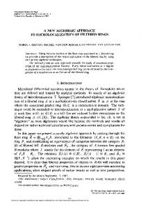
1. A Mathematical Introduction to Aharonov-Bohm Effect The Aharonov-Bohm effect, demonstrates that it is not possible to describe all electromagnetic phenomena in terms of the field strength only. This effect is observed for example in an electron double slit experiment. Let us consider the double slit experiment sketched in figure 1. The magnetic field B at the center is confined to a narrow tube such that the electrons move in a field-free region.

Figure 1. The Aharonov-Bohm effect

This implies that classically one would not expect to see any effect, since fields interact only locally. It turns out however that there is a quantum mechanical effect. Due to the vector potential A , the electron interference pattern on the screen, on the right, shifts over a distance proportional to the magnetic flux [1]. Free particles in a magnetic field are

described by the Schrödinger equation. This method of splitting the wave function in two parts is a semi-classical approximation since we ignore the effects of diffraction. Aharonov and Bohm in their original paper [2] also solved the problem without splitting the wave function in two parts. Moreover, Lee Page [3] has solved the problem of a free charged particle moving in a magnetic field and he found a solution which is finite in the origin. In addition to above viewpoints, the Aharonov–Bohm effect can be understood from the fact that we can only measure absolute values of the wave function [3-5]. However, by gauge invariance, it is equally valid to declare the zero momentum eigenfunction to − iφ x be e ( ) at the cost of representing the i -momentum operator (up to a factor) as ∇i ≡ ∂ i + i ( ∂ iφ ) , i.e. with a pure gauge vector potential A = dφ [6,7]. Therefore, the Aharonov–Bohm effect manifests itself as a connection with flat space and topologically nontrivial [8-10]. Effects with similar mathematical interpretation can be found in other fields. For example, in classical statistical physics, quantization of a molecular motor motion in a stochastic environment can be interpreted as an Aharonov–Bohm effect induced by a gauge field acting in the space of control parameters [11,12]. In this paper however, we deal with a different mathematical approach to the generalized Aharonov-Bohm effect, namely the algebraic operator method. This method, introduced in [13], provides the discrete spectrum and the energy level of the quantum Aharonov-Bohm effect, applying a SU(2) dynamical invariance algebra. This method has been generalized for coupled Aharonov-Bohm-Coulomb effects

American Journal of Modern Physics 2015; 4(2): 44-49

[14] and also for oscillating systems [15]. Therefore, it appears to be a powerful mathematical method for rederivations and generalizations of quantum phenomena. Note also that, such approaches have been considered in treating Schrödinger equation (for example see [16]). The paper is organized as follows: In section 2 we review the traditional way of solving three dimensional Schrödinger equation and we treat the Aharonov-Bohm effect using the wave functions. In section 3, we introduce the so-called operator algebra and revise the foundations of the Aharonov-Bohm effect in a Coulomb field. We conclude in section 4 and also make an outlook.

2. Generalized Aharonov-Bohm (AB) Effect

2πρ

δ (ρ)

(7)

α Hˆ = −∇ 2 + VA ( r , θ ) − . 2

(8)

Finally, the radial part of Schrödinger equations in spherical coordinates and in the presence of AB potential will be d 2 R 2 dR l0 ( l0 + 1) α  + − R +  + E  R = 0, 2 2 dr r dr r 2 

 d 2 u  −l0 ( l0 + 1) α + + + E  u = 0, 2 2 dr r r  

(9)

(10)

where u ( r ) = rR ( r ) . According to this, the effective potential would be

 α l ( l + 1)  Veff = −  − + 0 0 2 . r  r  Note that −

α

(11)

is a Coulomb potential, while

l0 ( l0 + 1)

is a r r2 repulsive one. Moreover, one can redefine the radial solution in the following form:

R ( r ) = e− ρ ρ 0

l H (ρ )

(2)

,

(12)

H ( ρ ) = ∑ an ρ n

(13)

where

with δ ( ρ ) as the Dirac delta function, for which the flux is

∞

given by

n =0

∫ B.ds =

.

(3)

and

an +1 2n + 2l0 + 2 − λ = . an ( n + 1)( n + 2l0 + 2 )

Moreover, the Schrödinger equation in the presence of an electric charge e′ and the AB potential is 2 α   −i∇ − e′ A − 2 ψ = Eψ ,  

(

)

(4)

A.∇ψ =

∂ψ . 2π r 2 sin 2 θ ∂φ

Therefore the leading term could be found at the extent points which near e ρ and at infinity behaves like ρ l0 . In equation changes to

(5)

According to axial symmetry, the energy spectrum is independent of the azimuth quantum number m , therefore one can write the m -dependent part as

ψ ( r ,θ ,φ ) = R( r ) y(θ ) eimφ .

(14)

other points, the leading term is named H ( ρ ) . So our

Or in spherical coordinates

So

im ψ. 2π r 2 sin 2 θ

Accordingly, the Schrödinger Hamiltonian becomes:

(1)

where is the flux. The magnetic field in the cylindrical coordinates reads as

B=k

A.∇ψ =

Which turns out that could be rearranged to

In this section, we deal with the Schrödinger equations for a charged particle e′ which is subjected to another Coulomb potential, exerted by another charge e , and the following AB potential (our approach is based on what has been developed in [13]):

  Ar = Aθ = 0     Aφ = 2π r sin θ 

45

(6)

 dH  λ − 2 − 2l0  d 2 H  2l0 + 2 + − 2 +  H ( ρ ) = 0, ρ dρ2  ρ  dρ  

(15)

which has to be solved. Using the recursion relation an +1 2n + 2l0 + 2 − λ , one can find = an ( n + 1)( n + 2l0 + 2 )

λ = 2 ( n2 + l0 + 1)

(16)

46

Farrin Payandeh: An Algebraic Operator Approach to Aharonov-Bohm Effect

As it is seen, the effect of the AB Coulomb potential in the Schrödinger equation, is to change the quantum orbital

and

n0 = n2 + l0 + 1

(17)

for which n2 = 0,1, 2,... and l0 = 0,1, 2,..., n0 − 1 . Therefore

n0 ≥ l0 + 1 or l0 ≥ n0 − 1 . This may lead us to conclude

( n0 )min

= 1 . Also the energy eigenstates are derived as E=−

α2 2 0

4n

,

n0 = 1, 2,... .

(18)

number, l. This term is added to a e′

2π

shift in the orbital number. Now if we set β → 0 , the flux vanishes and therefore l0 → l = n1 + | m | , which is the angular momentum of Hydrogen electron in usual situation, whereas in the presence of a superconductor in the region of B = 0 , we have l0 = n1 + m − e′

2π

Schrödinger

Now let us turn to the angular part of Schrödinger equation. In spherical coordinates we have 2  1 ∂   ∂y  − ( m + β )   = −l0 ( l0 + 1) , (19) θ y ( )  sin θ + ∂θ  sin 2 θ y (θ )  sin θ ∂θ   

1

and this would be the

. In this problem we solved the

equation

with

α where Hˆ = −∇ 2 + VA ( r ,θ ) + VA ( r , θ ) = 2

the β r 2 sin 2 θ

Hamiltonian .

On the other

hand all these results could be obtained for Hˆ = −∇ 2 − α (or H eff

2 α = p 2 − ), but upon this condition that instead of the 2

quantum orbital number l , we use l0 . In other words, instead

which can be rewritten as 2  γ2  + l0 ( l0 + 1) − (1 − x ) dxd 2 − 2 x dy  y ( x ) = 0, (20) dx  1 − x2  2

where γ 2 = ( m 2 + β ) and x = cos θ . The above equation is the associated Legendre differential equation which can be transformed to the Hypergeometric differential equation, using the change in variables. Here we just point out the important results of both methods. In the change in variables method, we put

l ( l + 1) of the centrifugal term l ( l +2 1) , we use 0 0 2 . Indeed, the r r

above results show that the effect of the coulomb potential

r in the Schrödinger equation is that to shift the quantum magnetic number m by a value of e′ , i.e. changes | m | to 2π m−

e′ . Moreover, the number of degeneracies are derived 2π

to be

γ

y ( x ) = ( x 2 − 1) 2 z ( x ) ,

e′   w = 2  l0 +  + 1, 2π  

(21)

and

α

(26)

or

t=

1+ x . 2

e′   w = 2  n0 +  − 1. 2π  

(22)

(27)

Then we get t (1 − t )

d2z dz + ( γ + 1) − ( 2γ + 2 ) t  − ( γ − l0 )( γ + l0 + 1) z = 0, (23) dt 2  dt

which is the Hypergeometric differential equation. According to this, we will have the following spectrum:

γ = ( m2 + β ) 2 = m −

e′F , 2π

n0 = 1 + n1 + n2 + m −

e′F , 2π

1

E=−

3. Solving Schrödinger Equation in AB Potential, Using Operator Algebra The Schrödinger equation for a linear oscillator could be written as

− (24)

d mω   a = dx + ℏ x   a † = − d + mω x  dx ℏ

e′F  1 + n1 + n2 + m −  . 4  2π 

Finally, the solution of our differential equation will be

y ( x) =

n1 = l0 − γ

∑ n0

(γ − l0 )n (γ + l0 + 1)n 2n n !( γ + 1)

(x

γ

2

− 1) 2 (1 − x ) . (25) n

(28)

Defining the following operators:

−2

α2 

ℏ 2 ∂ 2ψ 1 + mω 2 x 2ψ = Eψ . 2m ∂x 2 2

we get

(29)

American Journal of Modern Physics 2015; 4(2): 44-49

2  † d 2 mω  mω  + x  aa = − 2 + ℏ  ℏ  dx  .  2 d 2 mω  mω   †  a a = − dx 2 − ℏ +  ℏ x    

1  E =  n +  ℏω . 2  (30)

and hence a † aψ n = 0. This may lead us to

ℏ2 1 ψ n′′+1 + mω 2 x 2ψ n +1 + ( n + 1) ℏωψ n +1 = Eψ n +1 , 2m 2 (31) 2 ℏ 1 − ψ n′′ + mω 2 x 2ψ n + nℏωψ n = Eψ n . 2m 2 −

 1 mω x 2  2 ℏ

ψ n = α exp  −

 , 

(35)

where

α=

πℏ . mω

(36)

3.1. Solving Schrödinger Equation for Three Dimensional Oscillator in Spherical Coordinates

These could be simplified to

a † aψ n =

(34)

To obtain the ground state itself, we must have aψ n = 0

Accordingly, one can rewrite the Schrödinger equations for two energy levels in neighborhood, in terms of the above operators. We have

aa †ψ n +1 =

47

2m  1   E −  n +  ℏω ψ n +1 , 2  ℏ  2  

(32)

2m  1   E −  n +  ℏ ω ψ n . ℏ 2  2  

One can show that the wave functions ψ n and ψ n +1 satisfy the following recursion relations, according to the operator equations (32):

 ℏ2 a †ψ n +1 ψ n =  1    2 m  E −  n +  ℏω   2     .  ℏ2  aψ n ψ n +1 =  1    2m  E −  n +  ℏω  2    

In spherical coordinates, the Schrödinger equation can be written in the following way:

ψ = rR (r ), −ℏ 2 ℏ 2 l ( l + 1) 1 ψ ′′ + mω 2 r 2ψ + ψ = Eψ . 2m 2 2m r 2

(37)

We define two appropriate operators as

d mω l + r− , dr ℏ r d mω l a † (l ) = − + r− . dr ℏ r

a (l ) =

(33)

(38)

Accordingly, one can calculate a † a and aa † . Like usual one-dimensional harmonic oscillator, we shift the potential by ( n + 1) ℏω and write the corresponding Schrödinger

Also according to (32), the energy levels of the system would be

equation for the shifted potential. We have

2(n + 1)mω l (l + 1) 2mE  mω  −ψ ′′n +1,l +  r  ψ n +1,l + ψ n +1,l + 2 ψ n +1,l = 2 ψ n +1,l , ℏ r ℏ  ℏ  2

(39)

2nmω l (l − 1) 2mE  mω  ψ n ,l −1 + 2 ψ n ,l −1 = 2 ψ n,l −1 . −ψ ′′n ,l −1 +  r  ψ n ,l −1 + ℏ r ℏ  ℏ  2

the state n = 0 and l = l . In such state we will have

According to (41) and (42) one can infer

a (l ) a † (l )ψ n +1,l = a (l )a (l )ψ n ,l −1 †

2m  1   E − ℏω  n + l +  ψ n +1,l , 2  ℏ  2  

2m  1   = 2  E − ℏω  n + l +  ψ n ,l −1 . 2  ℏ  

ψ n +1,l = (40)

For the rhs of the second relation in (40) to be vanished, we must lower the states in ψ n ,l −1 to reach ψ 0,l , since the zero state and its corresponding momentum l , are constructing the ground state of a harmonic oscillator in a potential, shifted by a nℏω . We do this for a sequence of potentials until we reach

ψ n ,l −1 =

ℏ2  1   2 m  E −  n + l +  ℏω  2    ℏ2  1   2 m  E −  n + l +  ℏω  2   

Equation (44) may result in

a(l )ψ n ,l −1 , (41)

a (l )ψ n +1,l . †

48

Farrin Payandeh: An Algebraic Operator Approach to Aharonov-Bohm Effect

ψ 0,l =

ℏ2

ℏ2

  3  2 m  E −  l +  ℏω   2  

  7  2 m  E −  l +  ℏω   2  

…

ℏ2  1   2 m  E −  l + 2 n +  ℏω  2   

(42)

× a† (l + 1)a † (l + 2) … a† (l + n) ψ n ,l + n .

Therefore, one must put l → l + n + 1 in the second of (40) to get

a † (l + n + 1)a† (l + n + 1)ψ n ,l + n = 0 = hence

1  E = ℏω  l + 2 n +  . 2 

(44)

3.2. The Parabolic Counterpart In parabolic coordinates, the Schrödinger equation can be written as

(

−u′′ = i Eζ

)

2

1 e′  − 1 − 4 m − 4 2π  + u = cu. 2

ζ

(45)

In this case, the appropriate operators can be defined as d l + i Eζ − , dζ 2 d l A† (l ) = − + i Eζ − . dζ 2 A(l ) =

(46)

The one dimensional harmonic oscillator has to be solved in a potential, shifted by a 4i E (n + 1) . The same process as it is in subsection 3.1, will result in E=−

α2 

−2

e′   1 + n1 + n2 + m −  , 4  2π 

2m  1   E − ℏ ω  l + 2 n +  ψ n , l + n , 2  ℏ 2  

(43)

The method applied in this paper, has been also of interest in generalized Aharonov-Bohm effect in Coulomb and oscillating systems [14, 15], scattering states [17], bound states of Schrödinger equation [18, 19], and in a graphene ring [20]. Therefore, Aharonov–Bohm–Coulomb problem, which was the main subject of investigation of this paper, can be regarded in two different ways. One by use of the traditional method of solving Shrodinger eqaution for the scalar coupling and the other by applying the operator algebra, introduced in section 3, for most important coordinate systems. It has been found that, the energy spectrum of the system demonstrates that the degeneracies are diminished and it is clear from the spectrum of the AB potential. It is therefore of interest for further works, to generalize this algebraic operator method, for some other quantum effects like the ones in which the zero state energy (or the vacuum energy) is the cause of physical phenomena like the Casimir effect. In this case, the operators should be generalized to Dirac particles and their creation-annihilation process should be included as well. However, the mentioned graphene ring in reference [20] is a good example of such generalization. Therefore it seems that the doors are open for further insights into this methodical approach.

(47)

which is the same result as it is expected from (45). Here instead of solving the differential equation, the operator method has been used.

4. Conclusion Our aim in this paper was the investigation of the captured magnetic flux, when it is applied on the energy spectrum of a bounded charged particle, in the presence of external oscillator or coulomb potentials. As it was shown, the energy spectrum and their corresponding quantum numbers are e′ shifted by a , and also the degeneracies are decreased. 2π Indeed, applying the operator method, we could anticipate this phenomenon, which is in agreement with the usual mathematical methods.

References [1]

S. Gasiorowicz: Quantum physics, John Wiley (1974)

[2]

Y. Aharonov, D. Bohm: Physical Review 115: 485–91 (1959)

[3]

L. Page: Physical Review 36, 444 (1930)

[4]

A. Batelaan, A. Tonomura: Physics Today 62 (9): 38-43 (2009)

[5]

E. Sjöqvist: Physical Review Letters 89 (21): 210401 (2002)

[6]

W. Ehrenberg, R.E. Siday: Proceedings of the Physical Society. Series B 62: 8–21 (1949)

[7]

F.D. Peat: Infinite Potential: The Life and Times of David Bohm, Addison-Wesley. ISBN 0-201-40635-7 (1997)

[8]

Y. Aharonov, D. Bohm: Physical Review 123: 1511–1524 (1961)

[9]

M. Peshkin, A. Tonomura: The Aharonov–Bohm effect. Springer-Verlag. ISBN 3-540-51567-4 (1989)

American Journal of Modern Physics 2015; 4(2): 44-49

49

[10] L. Vaidman: Physical Review A 86 (4): 040101 (2012)

[16] M. R. Brown, B. J. Hiley: arXiv:quant-ph/0005026v5

[11] R. Feynman: The Feynman Lectures on Physics 2, pp. 15–5 (1964)

[17] S. Sakoda, M. Omote: Advances in Imaging and Physics 1, 110, 101–171 (1999)

[12] V.Y. Chernyak, N.A. Sinitsyn: Journal of Chemical Physics 131(18): 181101 (2009)

[18] M. Aktaş: International Journal of Theoretical Physics 48, 7, 2145–2163 (2009)

[13] H.D. Doebner, E. Papp: Physics Letters A 144, 8–9, Pages 423–426 (1990)

[19] M. Aktaş: Journal of Mathematical Chemistry 49, 9, 1831– 1842 (2011)

[14] Gh. E. Draganascu, C. Campigotto, M. Kibler: Physics Letters A 170, 6, 339–343 (1992)

[20] E. Jung, M-R. Hwang, C-S. Park, D. Park: Journal of Physics A: Mathematical and Theoretical 45, 5, 055301 (2012)

[15] M. Kibler, C. Campigotto: Physics Letters A 181, 1, 1–6 (1993)

H.

Electron