A variable is local if it occurs in a clause body but not in its head. ... In Section 3, we present a preliminary adjustment of the variable occurrences. Section 4 is ...
An Algorithm for Local Variable Elimination in Normal Logic Programs ´ Javier Alvez and Paqui Lucio Faculty of Computer Science, Basque Country University, San Sebasti´ an, Spain. {jibalgij,jiplucap}@si.ehu.es
Abstract. A variable is local if it occurs in a clause body but not in its head. Local variables appear naturally in practical logic programming, but they complicate several aspects such as negation, compilation, memoization, static analysis, program approximation by neural networks etc. As a consequence, the absence of local variables yields better performance of several tools and is a prerequisite for many technical results. In this paper, we introduce an algorithm that eliminates local variables from a wide proper subclass of normal logic programs. The proposed transformation preserves the Clark-Kunen semantics for normal logic programs.
1
Introduction
Local variables are very often used —as auxiliaries— to store intermediate results in logic programs. Their values are passed from one atom to another in a clause body, but they are not lifted to the head. Whilst they are useful in practical logic programming, the occurrence of local variables could cause inefficiency or even prevent the satisfaction of some properties. In the area of negation in logic programming, several results are restricted to local variable free (lvf, for short) programs or are less efficiently applicable when local variables are present. For instance, local variables lead to floundering problems in negation as failure [8]. In addition, their presence prevents completeness results for more recent techniques like intensional negation [5] and other transformational negation techniques [20, 25]. In several computational mechanisms proposed for constructive negation [7, 6, 11, 23, 2], local variables force one to deal with universal quantification, which is not easy to compute in an efficient manner. Other logic programming areas where local variables lead to technical problems are related to compilation, memoization, static analysis, program approximation by neural networks etc. Moreover, in equational logic programming, local variables cause problems since, in their presence, narrowing may become incomplete. In [12], some transformations of definite (equational) logic programs into lvf ones are presented. Unfortunately, these methods do not preserve failure. It is well known that every computable function can be computed by a definite logic program [3, 24]. Besides, the program built in [24] is an lvf definite program. Therefore, from the theoretical point of view, the function that is computed by any given normal logic program (according to the Clark-Kunen semantics) can
also be computed by an lvf definite program (in PROLOG). The question is how to automatically generate an lvf program from any given program with local variables. In particular, the lvf program given in [24] simulates the computation of a universal Turing machine over the Turing machine that computes the recursive function. This is not the program that we try to generate by transformation. Besides, each lvf normal program can be transformed into a definite one (see, for instance, [5]). Hence, the automatic removing of local variables from normal programs is a plausible and encouraging goal. In this paper, we present an algorithm for eliminating the local variables from normal logic programs while preserving the Clark-Kunen semantics. This method is applicable, in particular, to the class of well-moded logic programs ([9, 10, 19]). We explain the algorithm, prove its correctness and give illustrative examples. Outline of the paper. In the next section, we fix notation and terminology. In Section 3, we present a preliminary adjustment of the variable occurrences. Section 4 is devoted to partition the arguments of literals depending on the local variables, called mode, and to the notion of tail recursion w.r.t. a mode. In Section 5, we explain how to eliminate the local variables of a literal and the necessary conditions for doing this. The transformation to tail recursion w.r.t. a mode is shown in Section 6. In Section 7, we discuss the algorithm and its termination. Finally, we summarize conclusions and briefly discuss related work.
2
Preliminaries
We assume that the reader is familiar with the basic concepts and notation of logic programming, see e.g. [4]. In this section, we recall some basic terminology and introduce some notational conventions used throughout the paper. A bar is used to denote tuples, or finite sequences, of objects. For example, x denotes an n-tuple of variables x1 , . . ., xn. Throughout the paper, tuples of variables are assumed to be pairwise distinct. As a consequence, we treat them as sets and use the constant ∅ and the operators r (set difference), ∪ and ∩ for tuples of variables with their usual meaning over sets. However, tuples of terms and tuples of literals may have repeated elements. In such cases, concatenation of tuples is denoted by the infix operator · and h i stands for the empty tuple. In clauses, we split the variables into global and local. A variable is local in a clause if it occurs in its body but not in its head. Otherwise, it is global. For α which is a clause —or any syntactic object inside a clause like atom, term, etc— we denote by LVar(α) (GVar(α)) the set of local (global) variables in α. An lvf clause/program is a clause/program free of local variables. A literal is either an atom p(t) (positive literal) or a negated atom ¬p(t) (negative literal), where p and ¬p are the predicate (symbol) of the literal and t is a tuple of terms. We usually denote literals by L(t), M (t), N (t), . . . and L, M , N , . . . are used to denote the predicate of a literal. In a literal, when we do not need to specify the arguments, we simply omit the tuple of terms, and then
L, M , N , . . . denote a literal. Throughout the paper, the context always makes it clear whether a capital letter stands for a literal or a predicate symbol. Our program transformations preserve the Clark-Kunen semantics of normal programs, which is given by Clark’s program completion [8] interpreted in threevalued logic [13]. Note that the logical Clark-Kunen semantics is independent of the order in which the literals appear in the clause bodies. Given a normal program P and a predicate symbol p, DefP (p) is the set of all clauses from P whose head literal begins with p. From Clark’s completion, we have that ¬p(x) ↔ ¬ϕ where ϕ is the disjunction of the body clauses, which are existentially quantified on its local variables. If DefP (p) has no local variables, then ¬p(x) ↔ ¬ϕ can be easily reduced to a set of clauses that have a normal body and a negative head.1 In this case, we say that this is a normal definition called DefP (¬p). Otherwise, the universal quantification in clauses with head ¬p(x) can not be avoided and we say that DefP (¬p) is a complex definition. In our transformations, only normal definitions are handled. Complex definitions are delayed until they become normal or, otherwise, they are delayed forever. We make use of the fold/unfold transformation system described in [17] (see also [15]) where equivalence w.r.t. the Clark-Kunen semantics for definite programs is ensured by forbidding unfolding on direct recursion and requiring that a clause C should be folded with another clause, different from C, taken from the current program. Besides, this result can be extended to normal programs with the proviso that only normal (not complex) definitions of negated predicates are used. However, the fold/unfold technique is not powerful enough to prove some of our results and we complement it with direct induction on the bottom-up computation of the Clark-Kunen semantics. Given a program P and two predicates L and M , we say that M directly depends on L if L occurs in DefP (M ). By the reflexive transitive closure of this relation, we obtain the set DpdP (L) of all predicates on which L depends. Besides, we define the set of all mutually recursive predicates with L by: MRP (L) = {M | M ∈ DpdP (L) and L ∈ DpdP (M )}. The induced equivalence relation —given by (L, M ) ∈ R ⇐⇒ L ∈ MRP (M )— partitions the set of all predicates into a finite number of equivalence classes. Classes are MRP (L) where L is the class representative predicate. Then, the set consisting of all the equivalence classes (or factor set) can be partially ordered by the following relation: MRP (L) � MRP (M ) ⇐⇒ There exists N ∈ MRP (L) and Q ∈ MRP (M ) such that N ∈ DpdP (Q). Moreover, given a program P , its set of mutually recursive classes does not contain any infinite decreasing chain with respect to �. That is, � is a wellfounded order. For technical reasons, we need to distinguish the body literals 1
Of course, disequality is needed.
that are mutually recursive with the clause head. Hence, when convenient, a clause will be written in the following Dpd-form: H
1
2
n
L , K1 , L , . . . , L , Kn, L
n+1
to denote that Ki ∈ MRP (H) for each 1 ≤ i ≤ n and M 6∈ MRP (H) for each i M ∈ L and each 1 ≤ i ≤ n + 1. Note that n = 0 when no body literal belongs i to MRP (H). Besides, every L could be an empty tuple. In what follows, we assume a program, always called P , that is being transformed into an lvf program. We would like to emphasize that, although our method chooses some ordering on the clause bodies and the target programs depend on that ordering, we always preserve the Clark-Kunen semantics.
3
Local-Regulation
Local-regulation (LR, for short) is a preliminary treatment of the variable occurrences in the clause bodies. Roughly speaking, it is an adjustment for enabling local variable elimination. First, we define some syntactic conditions, called termapartness, and show that it can be achieved by program transformation. Definition 1. Let L(t) be an n-ary literal in a given clause H M, L(t), N and x ⊆ Var(L(t)). The variables x are term-apart in L(t) iff for every 1 ≤ i ≤ n (at least) one of the following two conditions holds: (a) Var(ti ) ∩ x ∩ Var(M ) = ∅ (b) Var(ti ) ∩ x ∩ Var(N ) = ∅.
t u
For example, given the clause h(x) p(x), q(x, f(x, y), y), ¬ h(y), the variables (x, y) are not term-apart in q(x, f(x, y), y) due to the term f(x, y) in the second argument, but each variable individually is term-apart in that literal. The intuition behind term-apartness is that it allows us to partition the terms t of a literal L(t) in two tuples t1 and t2 such that the variables that occur in t1 (t2) only occur in the left-hand side literals M (right-hand side literals N ). This partition facilitates the dataflow analysis of the clause. Lemma 1. Every normal program P can be transformed into a Clark-Kunen equivalent normal program P 0 such that all its variables are term-apart in the literals occurring in P 0. Proof. Let x ⊆ Var(L(t)) in a clause C = H M , L(t), N ∈ P such that w = Var(ti ) ∩ x ∩ Var(M ) 6= ∅ and Var(ti ) ∩ x ∩ Var(N ) 6= ∅ for some i. We define a new predicate p by D = p(z · w · w) L(z) and substitute the clause 0 C0 = H M , p(t · w · w0), N [w0/w] for C, where w0 is a tuple of fresh variables 0 and t is obtained by replacing ti with ti[w0/w] in t. In the resulting program, D is an lvf clause since only a literal occurs in its body and, besides, we have that Var(t0i ) ∩ x ∩ Var(M ) = ∅ in the clause C 0 . Furthermore, it is easy to see 0 that the new literal p(t · w · w0 ) in C 0 will not be affected by any subsequent transformation. After this process, equivalence is preserved since we obtain the 0 program P by unfolding the new literal p(t · w · w0 ) in C 0 with the clause D. u t
Now, we formulate the condition of local-regularity on clauses and extend it to programs in an obvious way. Definition 2. A clause C: H
1
2
n
n+1
L (r1 ), K1 (s1), L (r2 ), . . . , L (rn), Kn (sn), L
(r n+1)
in Dpd-form is local-regular iff n = 0 or it satisfies the following two conditions: (a) LVar(Ki (si )) are term-apart in Ki (si ) for every 1 ≤ i ≤ n (b) every local variable occurs in si−1 · ri · si for some 1 ≤ i ≤ n + 1 and does not occur anywhere in the clause (by convention, s0 = sn+1 = h i). A program P is local-regular iff every clause C ∈ P is local-regular.
t u
Next, we show a method to transform any program into a local-regular one. Lemma 2. Every normal program P can be transformed into a Clark-Kunen equivalent local-regular normal program P 0. Proof. Due to Lemma 1, we can always transform P into an equivalent program that satisfies the first condition. Therefore, we only focus on the second condition. 1 n+1 n+1 Let C = H L (r1 ), K1 (s1 ), . . . , Kn(sn ), L (r ) ∈ P be a clause in Dpd-form such that the leftmost occurrence of a local variable y that violates the i second condition is either in Ki−1(si−1) for 2 ≤ i ≤ n or in L (ri ) for 1 ≤ i ≤ n i and let C be rewritten as H M , L (ri ), Ki (si ), N . Then, we replace C with: C0 = H
i
M , L (ri ), pi (si · y · y0 ), N [y0 /y]
where y0 is a new local variable and pi is a new predicate defined by the clause D = pi (z · x · x) Ki (z). Now, y satisfies the second condition since it exactly i occurs in the tuple of literals Ki−1(si−1) · L (ri ) · pi (si · y · y0 ) in C 0. The iteration of this process ends because either the number of local variables that violate the condition decreases (that is, y0 satisfies it) or y0 occurs closer to the end of the clause body in C 0 than y in C: the leftmost occurrence of y is either in i Ki−1(si−1) or in L (ri ) in the clause C whereas the leftmost occurrence of y0 is in pi(si ·y·y0) in the clause C 0. Also, the new predicate pi is mutually recursive to H and, therefore, the clause C 0 is in Dpd-form. Besides, it is easy to see that the first condition of local regulation is always preserved by the above transformation. We have that the resulting program P 0 is equivalent to P because we obtain P by unfolding the new literals in P 0. t u The following example describes the transformation of a one-clause program into a local-regular program consisting of three clauses and using two fresh predicates. Example 1. Let us consider the following clause of some program P : E1.1 : p(f(x1 , x2))
q1(f(x2 , w1)), p1(g(w1 , w2)), q2(f(w2 , w1)), p2(g(w3 , x1)), q3(f(w2 , w3))
such that MRP (p) = {p, p1, p2}. The clause is not local-regular because the local variable w1 violates both conditions of Def. 2 and w2 violates the second one. Considering w1 , we define a new predicate p01 and replace E1.1 with the following clauses: E1.2 : p01 (z, w, w) p1 (z) E1.3 : p(f(x1 , x2)) q1(f(x2 , w1)), p01(g(w10 , w2), w1, w10 ), q2(f(w2 , w10 )), p2(g(w3 , x1)), q3(f(w2 , w3)) Now, w1 and w10 violate neither the first condition nor the second one. With regard to w2, its leftmost occurrence is in the literal p01 (g(w10 , w2), w1, w10 ). Therefore, we define a new predicate p02 and substitute the following clauses for E1.3: E1.4 : p02 (z, w, w) p2 (z) E1.5 : p(f(x1 , x2)) q1(f(x2 , w1)), p01(g(w10 , w2), w1, w10 ), q2(f(w2 , w10 )), p02(g(w3 , x1), w2, w20 ), q3(f(w20 , w3)) All the resulting clauses are local-regular. Thus, the source and target programs are shown to be equivalent by unfolding the literals of predicates p01 and p02 . u t
4
Input/Output Modes for Literals
Input/output modes were introduced in [16] and further extensively studied from many points of view and for many applications. In the classical view, the mode of a predicate indicates how its arguments will be used in the sense of identifying arguments which belong to the input and to the output. In this paper, in order to eliminate the local variable y, it might be necessary to consider as output the second argument in p(x1, y) and as input the second argument in p(x2, y). However, for the sake of clarity, we allow to assign a unique mode to each predicate. Hence, instead of assigning multiple modes to predicates, we consider a different but equivalent program where the predicates are conveniently renamed and different copies of the same predicate are provided, one for each different mode. Definition 3. A mode for an n-ary predicate L, denoted by m : L, is an n-tuple m ∈ {in, out}n , where the position i (1 ≤ i ≤ n) such that mi = in (mi = out) is considered as an input (output) position. t u Throughout this paper, we will use the following notation: Remark 1. Given a mode m for a predicate L and a literal L(t), the expression tI .m tO means the unique partition of t into the order-preserving subsequences consisting of the input (tI ) and output (tO ) arguments of L(t) according to m. Besides, the expression L(tI .m tO ) is called the IO-form of L(t), which implicitly represents m in L(t). Whenever the upper mode name m is irrelevant, we simply omit it and write L(tI . tO ). If (all or some of) the literals of a clause are in IO-form, then we say that the clause is in IO-form. From now on, the literals of any clause (in particular, in Dpd-form) can be written in IO-form. t u
Definition 4. Let C be a clause: H
M , L(t), K1 (u1 ), . . . , Kn (un), N
where: – y ⊆ Var(L(t)), – y ∩ Var(N ) = ∅, and – y ∩ Var(Ki (ui )) 6= ∅ for each 1 ≤ i ≤ n such that the variables y are term-apart in L(t). Then, the collection of modes {m : L, m1 : K1 , m2 : K2 , . . . , mn : Kn }, denoted by VarMode(C, L(t), y), is defined by: (a) mi = in if Var(ti ) ∩ y ⊆ Var(M ) and mi = out otherwise. (b) For each 1 ≤ j ≤ n: mji = in if Var(uji ) ∩ y 6= ∅ and mji = out otherwise.
t u
Note that, by the term-apartness of y, the variables in Var(tI ) ∩ y do not occur in K1 (u1), . . . , Kn (un). Example 2. Let C be the following clause in a program P : p(x1, x2)
q(f(x1 , y1 ), y1), r(y1 , f(x2 , y2)), r(x2, f(y2 , x2)), q(x1 , x1).
First, we need to rename the second literal r(x2, f(y2 , x2)), which is replaced with r0 (x2, f(y2 , x2)), and provide a copy of DefP (r) for the definition of the new predicate r0: C 0 = p(x1, x2)
q(f(x1 , y1 ), y1), r(y1 , f(x2 , y2)), r0(x2 , f(y2 , x2)), q(x1 , x1).
Then, the set of modes VarMode(C 0, r(y1 , f(x2, y2 )), (y1 , y2 )) is: {(in, out) : r, (out, in) : r0 } which yields the following IO-form of C 0: p(x1, x2)
q(f(x1 , y1), y1 ), r(y1
.
f(x2 , y2 )), r0(f(y2 , x2) . x2), q(x1 , x1).
By contrast, VarMode(C 0 , r(y1, f(x2 , y1)), x2) gives: p(x1, x2)
q(f(x1 , y1), y1 ), r(y1
.
f(x2 , y2 )), r0(x2 , f(y2 , x2) . h i), q(x1 , x1).
Note that we have not assigned a mode to the literals on q since r is not mutually recursive with the predicate q. t u Our intention is to eliminate the local variables that occur in the terms tO of a given L(tI .m tO ). For (in, out) : r (see Example 2), that variable is y2 . For this purpose, we must associate modes with the clauses in the definition of L according to m. That is, we first fix m as the mode for the head literal of each clause C in DefP (L). Then, taking into account the input/output partition of the head literal and the local variables of C, we associate a mode with every body literal of C that is mutually recursive with L.
Definition 5. Let m be the mode assigned to a predicate L and C be the following normal local-regular2 clause in Dpd-form: L(uI .m uO )
1
2
n
L (r1 ), K1 (s1 ), L (r2 ), . . . , L (rn ), Kn (sn), L
n+1
(rn+1 )
where each Ki (si ) is an ni -ary literal. Then, the mode for the clause C, denoted by ClauseMode(C, m), is given by the set of modes {m : L, m1 : K1 , . . . , mn : Kn }, where each mi is defined as follows: i−1 i in if LVar(sj ) ∩ LVar(r ) 6= ∅ or i LVar(sj ) = ∅ and (Var(sij ) ∩ Var(uI ) 6= ∅ or Var(sij ) ∩ Var(uO ) = ∅) mij = out otherwise for every 1 ≤ j ≤ ni . Besides, assuming that DefP (L) = {C1, . . . , Ck }, the mode for the definition of L, denoted by DefMode(P, L, m), is given by the set of clause modes {ClauseMode(C1, m), . . . , ClauseMode(Ck , m)}. t u Example 3. Let P be the following program: E3.1 : h(x) p(x, y), q(y), r(x) E3.2 : p(a, b) E3.3 : p(f(v), z) h(v), r(z) such that MRP (p) = {h, p}. Then, the set of modes VarMode(E3.1, p(x, y), y) yields the following IO-form for the clause E3.1: h(x)
p(x . y), q(y
h i), r(x)
.
Besides, since (in, out) is the mode for the predicate p, the set of clause modes DefMode(P, p, (in, out)) yields the following clauses: p(a . b) p(f(v) . z)
h(v
.
h i), r(z)
where the mode (in) is assigned to the predicate h. Finally, the set of clause modes DefMode(P, h, (in)) gives the clause: h(x . h i)
p(x . y), q(y
.
h i), r(x)
Note that, in this example, we have assigned a unique mode to the predicates h and p without renaming. u t Now, starting with a mode m assigned to a predicate L, we collect the modes that are assigned to all the predicates that are mutually recursive with L. Definition 6. Let m be the mode assigned to a predicate L in a program P . The relation ≺ is defined by: m : L ≺ m0 : M ⇐⇒ m0 : M ∈ DefMode(P, L, m). 2
By Lemma 2, we can assume local-regularity.
Besides, the mode for the predicates that are mutually recursive with L, denoted by ModeMR(P, L, m), is given by the least set of modes that contains the singleton {m : L} and is upwards closed with respect to the relation ≺. t u Example 4. In the program of Example 3, the set of modes ModeMR(P, p, (in, out)) is given by: {(in, out) : p, (in) : h } Note that, since we assign a unique mode to each predicate, we have that ModeMR(P, p, (in, out)) = ModeMR(P, h, (in)). t u Next, we present the notion of tail recursion, which is relative to a mode. Definition 7. The definition of a predicate L in a program P is tail recursive w.r.t. a mode m iff the following two conditions hold: (a) MRP (L) = {L} (b) the set of clause modes DefMode(P, L, m) yields clauses of the following two forms: (1 ) L(r I .m rO ) (2 ) L(sI .m z)
E F , L(s0I .m z)
where N 6∈ MRP (L) for each N ∈ E ·F and z is a tuple of fresh variables.
t u
This notion of tail recursion is more restrictive than the classical one. Intuitively stated, it means that, besides the fact that only the rightmost literal is headdependent, all the recursive calls return exactly the same value.
5
Elimination of the Local Variables of a Literal
When DefP (L) is tail recursive w.r.t. a mode, we are able to eliminate the local variables that occur in the output arguments of the selected literal L(t). This is done by substituting a set of clauses, called LVFP (C, L(t)), for the clause C. Definition 8. Let VarMode(C, L(t), y) yield the following IO-form for C: C=H
1 mn n M , L(tI .m tO ), K1 (u1I m. u1O ), . . . , Kn (un I . uO ), N
where y = LVar(L(t)) are term-apart in L(t) and y ∩ Var(N ) = ∅. If DefP (L) is tail recursive w.r.t. m, then LVFP (C, L(t)) consists of the following clauses: (a) One single clause of the form: H
M , p(tI , wI
.
uO , wO ), N
where uO = u1O ∪ . . . ∪ un O. (b) For each non-recursive clause L(rI .m rO ) p(rI σ, wI σ
.
v, wO σ)
E ∈ DefP (L), a clause:
1 mn n Eσ, K1 (u1I σ m. v1 ), . . . , Kn (un Iσ . v )
where σ = mgu(rO , tO ) and v = v 1 ∪ . . . ∪ v n . (c) For each recursive clause L(sI .m z) F , L(s0I .m z) ∈ DefP (L), a clause: p(sI , wI
.
F , p(s0I , wI
v, wO )
.
v, wO )
where p is a fresh predicate symbol, v is a fresh tuple of variables of the size of uO , wI = GVar(tO ) r GVar(tI · uO ) and wO = GVar(uI ) r GVar(tI · uO ). u t In the above definition, wI and wO are used to keep the links between literals through global variables. Note that, in the original clause C, the exact variables y occur in tO and ujI for 1 ≤ j ≤ n, but do not occur in LVFP (C, L(t)). Hence, y has been eliminated from C. Some occurrences of local variables could remain in the clauses of the form (b), but they are in literals that do not depend on the head. We will return to this matter for a discussion about termination. Theorem 1. Let LVFP (C, L(t)), L(t) and the clause C be as in Definition 8. The programs P and P 0 = P r {C} ∪ LVFP (C, L(t)) are Clark-Kunen equivalent. Proof. Let us assume that VarMode(C, L(t), y) yields the following IO-form: C:
H
1 mn n M, L(tI .m tO ), K1 (u1I m. u1O ), . . . , Kn (un I . uO ), N
where y = LVar(L(t)). A program P0 is obtained by introducing the new predicate p in P . In P0, p is defined by the single clause: D:
p(x, wI
.
z, wO )
1 mn n L(x .m tO ), K1 (u1I σ m. z 1 ), . . . , Kn(un Iσ . z )
where x, z 1, . . . , z n are tuples of fresh variables, the sets wI and wO are obtained as in Definition 8 and z = z 1 ∪ . . . ∪ z n . The programs P and P0 are trivially equivalent. Next, we obtain P1 from P0 by folding C using D: C0 :
H
M , p(tI , wI
u1O
.
uO , wO ), N
un O.
where uO = ∪ ... ∪ Then, the program P2 is obtained by unfolding the literal L(x . tO ) in the clause D. Since DefP (L) (and therefore, DefP1 (L)) is tail recursive w.r.t. m, it consists of clauses of the following two forms: T 1.1 : L(rI .m rO ) T 1.2 : L(sI .m z)
E F , L(s0I .m z)
and, hence, after the unfolding step, we get clauses of the form: 1
n
m n T 1.3 : p(rI σ, wI σ . z, wO σ) Eσ, K1 (u1I σ m. z 1 ), . . . , Kn (un Iσ . z ) 0 m 1 m1 1 mn n T 1.4 : p(sI , wI . z, wO ) F , L(sI . tO ), K1 (uI σ . z ), . . . , Kn(un Iσ . z )
where σ = mgu(rO , tO ). The programs P2 and P 0 are syntactically equal except 1 mn n for the clauses T 1.4, where L(s0I .m tO ), K1 (u1I σ m. z 1 ), . . . , Kn (un Iσ . z ) correspond with the literal p(s0I , wI . z, wO ) in the program P 0. It is easy (but tedious) to prove that P2 and P 0 are equivalent using induction on bottom-up computation of the Clark-Kunen semantics. The interested reader may find the details in [1]. Therefore, the programs P and P 0 are also equivalent. t u
Example 5. Let P be the following program: member(y, x1 ), ¬ member(y, x2 ) E5.1 : q(x1 , x2) E5.2 : member(x, [x| ]) E5.3 : member(x1 , [ |x2]) member(x1 , x2) In order to eliminate the local variable y, we first obtain the set of modes VarMode(E5.1, member(y, x1 ), y), that yields the following IO-form of E5.1: q(x1 , x2)
member(x1
.
y), ¬ member(y
.
x2 )
where the mode (out, in) is assigned to member. Besides, the set of clause modes DefMode(P, member, (out, in)) gives the following clauses: member([x| ] . x) member([ |x2] . x1 )
member(x2
.
x1 )
Since DefP (member) is tail recursive w.r.t. the mode (out, in), then the set of clauses LVFP (E5.1, member(y, x1 )) is a compound of: E5.4 : q(x1 , x2) p(x1 . x2 ) E5.5 : p([x| ] . z) ¬ member(x E5.6 : p([ |x] . z) p(x . z)
6
.
z) t u
Tail Recursive Transformation
We use the well known technique of the call stack for transforming recursion into tail recursion. The method in [21] also uses the call stack to convert a definite program into a continuation passing style program which, in particular, is a binary program (clauses have at most one literal in the body). We perform a similar, but simpler, treatment since our target program is not required to be binary. For the sake of readability, consider that the clauses to be transformed have (at most) two head-dependent literals in the body (see (1) below). Generalization to n literals is not difficult but unnecessarily complicates the description of the transformation we explain below. A given DefP (L), that is not tail recursive with respect to a mode m, is transformed into a new definition formed by the single clause: L(x .m z)
q(x, [cL] . z).
where q is a fresh predicate and cL is a constant that stands for L. This new definition is obviously tail recursive w.r.t. any mode (in particular w.r.t. m). Then, we use the original definition of L for providing a tail recursive definition of q w.r.t. the mode in q(x, [cL] . z), which is the extension of m by adding an input position. The definition of q is given by: – the single clause q(z, [ ] . z),
– plus, for each element m0 : K ∈ ModeMR(P, L, m) and each clause from DefP (K) (in Dpd-form): 0 K(tI m. tO )
1 2 1 2 3 L , K1 (s1I m. s1O ), L , K2 (s2I m. s2O ), L
(1)
the following four clauses: (i) (ii) (iii) (iv)
2 C C C q(tI , [cK |S] . z) q(tI , [w1 , cC 1 , w , c2 , w , c |S] . z) 1 q(tI , [w1, cC L , q(s1I , [cK1 |S] . z) 1 |S] . z) 2 q(s1O , [w2, cC L , q(s2I , [cK2 |S] . z) 2 |S] . z) 3 q(s2O , [wC , cC |S] . z) L , q(tO , S . z) 1
2
where z is a tuple of fresh variables, w1 = GVar(L ·s1I ), w2 = GVar(s1O ·L ·s2I ) 3 and wC = GVar(s2O · L · tO ) ∩ (w1 ∪ w2 ). The sets of variables in the stack are used to keep the links between literals through global variables. As defined, these sets are not minimal. A more sophisticated analysis would produce smaller sets of variables. Note that the fresh predicate q is used with tuples of terms of different sizes in the input arguments and, therefore, we are really defining several predicates, one for each arity. This is not a minor difference if we consider the dependences of predicates, especially in Definition 8. By contrast, the size of the tuple of fresh variables z is equal in all the clauses and it coincides with the number of output positions in m. Example 6. Let P be the following program: E6.1 : E6.2 : E6.3 : E6.4 :
k(a m . b) k(f(x1 ) m q(x1 m . f(x2 )) . x2 ) m q(x1 . x2 ) ¬ h(x1, x2) q(f(x1 ) m k(x1 m . y), q(g(y, x1 ) . f(x2 )))
m .
x2 )
where ModeMR(P, k, m) = {m : k, m : q} for m = (in, out). Since DefP (k) is not tail recursive w.r.t. m, a tail recursive definition of k w.r.t. m consists of the following clauses. First, the initial clauses: E6.5 : k(x m p(x, [ck] . z) . z) E6.6 : p(z, [ ] . z) where the constant ck stands for the predicate k. Since E6.1 is non-recursive, the above clauses (ii) and (iii) are not necessary (c1 corresponds with E6.1): E6.7 : p(a, [ck |S] . z) E6.8 : p(a, [c1|S] . z)
p(a, [c1|S] . z) p(b, S . z)
In the clause E6.2, there is one recursive literal. Hence, (iii) is not necessary: E6.9 : p(f(x1 ), [ck|S] . z) p(f(x1 ), [c21, c2 |S] . z) 2 E6.10 : p(f(x1 ), [c1|S] . z) p(x1, [cq |S] . z) E6.11 : p(x2 , [c2|S] . z) p(f(x2 ), S . z)
where c2 stands for the clause E6.2, c21 for the literal q(x1 . x2 ) and cq for the predicate q. The clause E6.3 is non-recursive (c3 corresponds to E6.3), then: E6.12 : p(x1 , [cq |S] . z) E6.13 : p(x1 , [c3|S] . z)
p(x1, [c3|S] . z) ¬ h(x1 , y), p(y, S
.
z)
Finally, the clause E6.4 has two recursive literals, where c4 , c41 and c42 respectively stand for the clause itself and the literals k(x1 . x2) and q(g(y, x1 ) . x2): E6.14 : E6.15 : E6.16 : E6.17 :
p(f(x1 ), [cq |S] . z) p(f(x1 ), [c41, x1, c42, c4|S] . z) 4 p(f(x1 ), [c1|S] . z) p(x1 , [ck|S] . z) p(f(x), [x1, c42|S] . z) p(g(x, x1), [cq |S] . z) p(x2 , [c4|S] . z) p(f(x2 ), S . z)
t u
It is easy to see that, in the above example, the transformed program uses the stack to simulate the computation of the original program for any goal. In general, the transformation works similarly for clauses with any arbitrary number of head-dependent body literals and it preserves the Clark-Kunen equivalence. The proof of this result is omitted for brevity and it can be found in [1]. Theorem 2. Let m be a mode for a predicate L in a program P . Then, the definition of L can be transformed into a Clark-Kunen equivalent definition that is tail recursive w.r.t. m. t u
7
An Algorithm for Elimination of Local Variables
Now, we present our algorithm —see Figure 1— for eliminating local variables. In previous sections, we have shown the basic transformations that our algorithm performs. These are: local-regulation (LR), elimination of a tuple of local variables (LVF) and tail-recursive transformation (TR). These three basic operations have different effects on the set of local variable occurrences in the transformed program. Sometimes, new local variables could arise in the new clauses and, at the same time, other local variables are erased. In this section, we show that it is possible to give decidable conditions that guarantee termination. Such conditions are concerned with the notion of a literal candidate, which we will make precise after a brief introduction of the algorithm itself. The algorithm outlined in Figure 1 first collects all the literals that contain some local variables in the set Lit(P ). Then, until Lit(P ) becomes empty, we select any literal L(t) from that set. Let assume that L(t) occurs in a clause C such that m is the mode assigned to the predicate L by VarMode(C, L(t), LVar(L(t))) and H is the literal in the clause head. On the one hand, if the selected literal is not a candidate (line 5), then we simply delete it from Lit(P ) and proceed to the next iteration. On the other hand, if L(t) is a candidate, then there are two main cases. If DefP (L) is tail recursive w.r.t. m (line 7), we substitute LVFP (C, L(t)) for C. Besides, we delete from Lit(P ) all the literals that occur in C and add to Lit(P ) all the literals from LVFP (C, L(t)) that contain some local variables. Otherwise, if the definition of L is not tail recursive w.r.t. m (line 12),
we transform DefP (L) into tail recursive w.r.t. that mode. Besides, we delete from Lit(P ) the literals that occur in DefP (L) and add to Lit(P ) the literals that contain some local variables in the new clauses. In the former case (line 7), we directly eliminate the subset of local variables from the clause C. In the latter case (line 12), the definition of L is adapted for fulfilling the condition of the first case. Note that, in the last case (line 12), the clause C is removed from P only if L depends on H, because DefP (L) = DefP (H). Therefore, we have to select a different candidate in the next step. Otherwise, L(t) can be selected as a candidate in the next step and the subset of local variables will be eliminated.
1 2 3 4 5 6 7 8 9 10 11 12 13 14 15 16 17 18
collect in Lit(P ) all the literals that contain some local variables while Lit(P ) 6= ∅ loop select a literal L(t) in a clause C = H M , L(t), N let m : L ∈ VarMode(C, L(t), LVar(L(t))) if L is not a candicate then delete L from Lit(P ) elsif DefP (L) is tail recursive w.r.t. m then substitute LVFP (C, L) for the clause C in P delete from Lit(P ) the literals in C add to Lit(P ) the literals in LVFP (C, L) that contain some local variables else transform DefP (L) into tail recursive w.r.t. m delete from Lit(P ) the literals in DefP (L) add to DefP (L) the literals in the new clauses that contain some local variables end if end loop Fig. 1. An Algorithm for Elimination of Local Variables
The algorithm in Figure 1 terminates when there is no candidate, although the resulting program may not necessarily be lvf. With regard to termination, the transformation LR introduces new local variables but, since local-regularity is preserved by the other two transformations, LR is applied only finitely many times. The transformation LVF does not introduce new local variables, but the local variables y to be removed could be only partially eliminated in some cases. In particular, a clause of the form (b) of Definition 8 could contain some variables from y. However, they necessarily occur in literals that do not depend on the clause head. This fact ensures termination because the set of all mutually recursive components of a program is well-foundedly ordered w.r.t. predicate dependencies. The transformation TR, explained in Section 6, could introduce new local variables, which could lead to non-termination problems through clauses (i) and (iv) (see Section 6). The problem arises when new local variables exactly occur in literals which depend on the clause head because, in that case,
the resulting definition is never tail recursive w.r.t that is given by VarMode with respect to the new local variables. Therefore, we would transform the definition of a predicate into tail recursive w.r.t. the corresponding mode infinitely many times. On the one hand, since clauses (i) are binary, they must be lvf in order to avoid that problem. On the other hand, let us illustrate the problem of clauses (iv) by the following example. Example 7. Consider the following program P : E7.1 : perfectsq(v) mult(y, y, v) E7.2 : mult(0, x, 0) E7.3 : mult(s(x1 ), x2, x3) mult(x1 , x2, y), sum(x2 , y, x3) To eliminate the local variable y in the first clause, VarMode(E7.1, mult(y, y, v), y) assigns the mode (out, out, in) to the predicate mult. Since DefP (mult) is not tail recursive w.r.t. (out, out, in), we transform the definition of the predicate mult as explained in Section 6. Then, the clause (iv) obtained from E7.2 is: q(0, [cE7.2|S] . z1 , z2)
q(0, y0 , S
.
z1, z2 )
where y0 is a new local variable that occurs in a literal that depends on the clause head. However, if the clause E7.2 is replaced with the following two clauses: E7.4 : mult(0, 0, 0) E7.5 : mult(0, s(x), 0)
mult(0, x, 0)
then, the respective clauses (iv) are lvf (therefore, not problematic): q(0, [cE7.4|S] . z1 , z2 ) E7.5
q(0, x, [c
|S] . z1 , z2)
q(0, 0, S
.
z1 , z2 )
q(0, s(x), S
.
z1 , z2 )
Note that the programs P and P r {E7.2} ∪ {E7.4, E7.5} are not Clark-Kunen equivalent. t u In order to avoid the termination problem, we can establish syntactic conditions to ensure that the clauses (i) are lvf and also that the new local variables of (iv) occur in literals which do not depend on the head. This is a sufficient condition for termination assuming that the literal selection rule (line 3 in Figure 1) is fair, although the resulting program might be not lvf. This condition is formally stated in the following definition. Definition 9. Let P be a program and N (u) be a literal in a clause C such that VarMode(C, N (u), LVar(N (u))) assigns the mode m to the predicate N and uI . uO is the unique partition of the tuple of terms u w.r.t. m. Then, the literal N (u) is called candidate iff: (a) LVar(N (u)) are term-apart in N (u) (b) DefP (K) is local-regular for every K ∈ MRP (N ) (c) LVar(uO ) 6= ∅
(d) for each element m0 : K ∈ ModeMR(P, N, m) and each clause in DefP (K) of 0 1 n n+1 3 n the form K(tI m. tO ) L , K1 (s1I . s1O ), . . . , L , Kn (sn : I . s O ), L 1 n (d.1) GVar(L · s1I · s1O · . . . · L · sn ) ⊆ GVar(t ) I I n+1 (d.2) GVar(tO ) ⊆ GVar(tI · L · sn ) O (e) DefP (K) is a normal definition for every K ∈ MRP (N ) t u The conditions (d.1) and (d.2) in the above definition respectively ensure that the clauses (i) and (iv) are not problematic. Note that, in Example 7, the literal mult(y, y, v) is not a candidate because (d.2) does not hold for E7.2 and n+1 mode (out, out, in), since GVar(tO ) = {x} and GVar(tI · L · sn O ) = ∅. On the contrary, the clauses E7.4 and E7.5 avoid this problem, because the former does not have any global variable, whereas for the latter GVar(tO ) = {x} and n+1 GVar(tI · L · sn O ) = {x}. Besides, the condition (e) ensures that, dealing with normal logic programs, the transformations LVF and LR are applicable to the involved definition. Note that the elimination of some local variables could turn a non-candidate literal into a candidate one when its complex definition becomes normal. We have verified that the algorithm in Figure 1 successfully works for most of the programs in Sterling and Shapiro [22] (about 35 definite programs and 6 normal programs). The interested reader may find them and their lvf version in the URL: http://www.sc.ehu.es/jiwlucap/LVF.html. Outstanding exceptions are the programs that use difference-lists. Let us give an example. Example 8. Let P be the following program: E8.1 : E8.2 : E8.3 : E8.4 :
flatten(x1 , x2) flatten dl(x1, x2 \ [ ]) flatten dl([ ], x \ x) flatten dl(x1, [x1|x2] \ x2 ) constant(x1), x1 6= [ ] flatten dl([x1|x2], x3 \ x4 ) flatten dl(x1, x3 \ y), flatten dl(x2, y \ x4)
that flattens a list of lists using difference-lists. The algorithm in Figure 1 cannot eliminate the local variable y in the clause E8.4. In order to eliminate y, the mode (in, out) : flatten dl is given by VarMode(E8.4, flatten dl(x1 , x3 \ y), y). However, the clause E8.2 does not hold the condition (d.2) in Definition 9 with respect to this mode. t u In spite of this drawback, our algorithm successfully eliminates all the local variables from a wide subclass of normal logic programs. That is, many pograms satisfy the conditions in Definition 9. In order to provide some more intuitition on the Definition 9, we would like to point out that any well-moded program ([9, 10, 19]) satisfy it. Roughly speaking, in a well-moded program, each predicate has assigned a unique mode such that the literals (in clause bodies) satisfy a left-to-right producer-consumer relation. For mostly well-moded clauses, that relation directly ensures the conditions (d.1) and (d.2) of Definition 9. Some 3
For technical reasons, we assume that s0O is the tuple tI
exceptions are due to the fact that we only assign modes to some predicates (the ones that are mutually recursive with the predicate in the clause head). This shortcoming can be avoided by requiring local-regulation (see Definition 2) in the global variables as it is required for the local ones. Notice that, in Example 7, the clauses E7.4 and E7.5 are well-moded. The first one is trivially well-moded because its body is empty and all the terms in its head are ground. In the clause E7.5, there is a well-moded producer-consumer relation since the literal in the clause body produces the output variable x of the head. Notice also that, on the contrary, the clause E7.2 cannot be well-moded because the output variable x is neither produced by the clause body (it is empty), nor is it also an input variable.
8
Conclusions and Related Work
We have introduced an algorithm that removes local variables from normal programs while preserving Clark-Kunen semantics and show that our algorithm eliminates all the local variables from a wide range of normal logic programs. However, it is still an open problem to decide whether any normal (or, even, definite) program can be transformed into an lvf one, despite the result of [24]. Since our transformation includes fresh symbols and new literals, a real implementation should clean up the target program to prevent a hypothetical performance deterioration. Superfluous literals can be removed by unfolding. Note that unfolding in an lvf program preserves the lvf feature. Furthermore, we can reduce the blow-up of new symbols and literals by keeping the original definition of predicates in the program, although their tail recursive versions are used for performing the local variable elimination. The work most closely related to our own is [21], where a continuation passing style (CPS, for short) transformation is introduced for definite programs. The CPS conversion is also related to both the call stack technique and the notion of mode. Moreover, the authors introduce the possibility of local variable elimination through CPS conversion and give a sufficient condition for successful elimination, called ground I/O condition, in a definite program. The ground I/O condition of a clause depends on some (arbitrary) mode for every predicate occurring in it. Anyway, there are marked differences in our approach and results. First, we deterministically assign one mode to each literal taking into account the local variables to be eliminated, whereas the transformation of [21] depends on an arbitrary mode. Second, we only manage the clauses that belong to the predicate definition (and the mutually recursive ones) of the selected literal. By contrast, in the approach of [21], the definition of all the literals in the affected clause are handled and all of them must satisfy the ground I/O condition. The aim of [18] is to yield more efficient SLD-computations of definite programs by the elimination of redundant computations caused by the so-called unnecessary variables. Local variables are a special kind of such unnecessary variables, because that method also considers as unnecessary those variables that occur more than once in the clause body (called multiple variables), even when they occur in the head. Different strategies for guiding the application of un-
fold/fold transformations are presented in order to eliminate such unnecessary variables. These strategies guarantee the complete elimination of unnecessary variables for a syntactically characterized subclass of definite programs. Other significant related work is [14], which introduces an algorithm, called RAF, for eliminating redundant arguments from definite programs. Actually, RAF is intended as a post-processing phase for program transformers, since automatic transformation produces many redundant arguments. Usually, local variables appear in redundant arguments. Hence, local variable elimination can be performed through a combination of some program transformation method (for instance, conjunctive partial deduction) and the RAF algorithm. This kind of system is closer in spirit to [18] than our own method. Acknowledgment: We would like to thank the anonymous referees for their valuable comments, which aided in improving the quality of this paper and in clarifying the presentation. This work was partially supported by the Spanish Project TIN2004-079250-C03-03.
References ´ 1. J. Alvez and P. Lucio. An algorithm for local variable elimination in normal logic programs. Technical Report LSI/TR 10-2005, Basque Country University, 2005. ´ 2. J. Alvez, P. Lucio, F. Orejas, E. Pasarella, and E. Pino. Constructive negation by bottom-up computation of literal answers. In SAC ’04: Proceedings of the 2004 ACM symposium on Applied computing, pages 1468–1475, New York, NY, USA, 2004. ACM Press. 3. H. Andr´eka and I. N´emeti. The generalized completeness of Horn predicate-logic as a programming language. Acta Cybern., 4:3–10, 1980. 4. K. R. Apt. Logic programming. In Handbook of Theoretical Computer Science, Volume B: Formal Models and Sematics (B), pages 493–574. Elsevier, 1990. 5. R. Barbuti, P. Mancarella, D. Pedreschi, and F. Turini. A transformational approach to negation in logic programming. J. Log. Program., 8(3):201–228, 1990. 6. P. Bruscoli, F. Levi, G. Levi, and M. C. Meo. Compilative constructive negation in constraint logic programs. In CAAP ’94: Proceedings of the 19th International Colloquium on Trees in Algebra and Programming, pages 52–67, London, UK, 1994. Springer-Verlag. 7. D. Chan. An extension of constructive negation and its application in coroutining. In NACLP, pages 477–493, 1989. 8. K. L. Clark. Negation as failure. In H. Gallaire and J. Minker, editors, Logic and Data Bases, pages 293–322, New York, 1978. Plenum Press. 9. P. Dembinski and J. Maluszynski. And-parallelism with intelligent backtracking for annotated logic programs. In SLP, pages 29–38, 1985. 10. W. Drabent. Do logic programs resemble programs in conventional languages? In SLP, pages 289–396, 1987. 11. W. Drabent. What is failure? an approach to constructive negation. Acta Inf., 32(1):27–29, 1995. 12. M. Hanus. On extra variables in (equational) logic programming. In ICLP, pages 665–679, 1995. 13. K. Kunen. Negation in logic programming. J. Log. Program., 4(4):289–308, 1987.
14. M. Leuschel and M. H. Sørensen. Redundant argument filtering of logic programs. In J. Gallagher, editor, Logic Program Synthesis and Transformation, Proceedings of LoPSTr ’96, Stockholm, Sweden, Lecture Notes in Computer Science 1207, pages 83–103. Springer-Verlag, 1996. 15. M. J. Maher. Correctness of a logic program transformation system. Technical Report RC 13496, IBM T.J. Watson Research Center, 1988. 16. C. S. Mellish. The automatic generation of mode declarations for prolog programs. Technical Report 163, Dept. of Artificial Intelligence, University of Edinburgh, Scotland, 1981. 17. A. Pettorossi and M. Proietti. Transformation of logic programs. In D. M. Gabbayand, C. J. Hogger, and J. A. Robinson, editors, Handbook of Logic in Artificial Intelligence and Logic Programming, Vol. 5, pages 697–787. Oxford University Press, 1998. 18. M. Proietti and A. Pettorossi. Unfolding - definition - folding, in this order, for avoiding unnecessary variables in logic programs. Theor. Comput. Sci., 142(1):89– 124, 1995. 19. D. A. Rosenblueth. Chart parsers as proof procedures for fixed-mode logic programs. In FGCS, pages 1125–1132, 1992. 20. T. Sato and H. Tamaki. Transformational logic program synthesis. In FGCS, pages 195–201, 1984. 21. T. Sato and H. Tamaki. Existential continuation. New Generation Comput., 6(4):421–438, 1989. 22. L. Sterling and E. Shapiro. The art of Prolog: advanced programming techniques. MIT Press, Cambridge, MA, USA, 1986. 23. P. J. Stuckey. Negation and constraint logic programming. Inf. Comput., 118(1):12–33, 1995. 24. S.-˚ A. T¨ arnlund. Horn clause computability. BIT, 17(2):215–226, 1977. 25. H. C. Wasserman, K. Yukawa, and Z. Shen. An alternative transformation rule for logic programs. In SAC ’95: Proceedings of the 1995 ACM symposium on Applied computing, pages 364–368, New York, NY, USA, 1995. ACM Press.