they are subdifferentiable. Proposition 1 The functions f and. ¯ f are semismooth. Proof: The sum and the minimum of semismooth functions are semismooth (see.
An algorithm for minimizing clustering functions
Adil M. Bagirov and Julien Ugon Centre for Informatics and Applied Optimization, School of Information Technology and Mathematical Sciences, University of Ballarat, Victoria, 3353, Australia
Abstract The problem of cluster analysis is formulated as a problem of nonsmooth, nonconvex optimization. An algorithm for solving the latter optimization problem is developed which allows one to significantly reduce the computational efforts. This algorithm is based on the so-called discrete gradient method. Results of numerical experiments are presented which demonstrate the effectiveness of the proposed algorithm.
1
Introduction
This paper develops an algorithm for minimizing the so-called clustering functions. Clustering is an important application area in data mining. Clustering is also known as the unsupervised classification of patterns. The cluster analysis deals with the problems of organization of a collection of patterns into clusters based on similarity. It has found many applications, including information retrieval, medicine etc. In cluster analysis we assume that we have been given a finite set A of points in the n-dimensional space IRn , that is A = {a1 , . . . , am }, where ai ∈ IRn , i = 1, . . . , m. There are different types of clustering such as partition, packing, covering and hierarchical clustering [20]. In this paper we will consider partition clustering, that is the distribution of the points of the set A into a given number q of disjoint subsets Ai , i = 1, . . . , q with respect to predefined criteria such that: 1) Ai 6= ∅, i = 1, . . . , q; 2) Ai
T
3) A =
Aj = ∅, i, j = 1, . . . , q, i 6= j; q S
Ai .
i=1
1
The sets Ai , i = 1, . . . , q are called clusters. The strict application of these rules is called hard clustering, unlike fuzzy clustering, where the clusters are allowed to overlap. In this paper we will consider the hard unconstrained clustering problem, that is no constraints are imposed on the clusters Ai , i = 1, . . . , q. An up-to-date survey of existing approaches to clustering is provided in [26] and a comprehensive list of literature on clustering algorithms is available in this paper. We assume that each cluster Ai , i = 1, . . . , q can be identified by its center (or centroid). Then the clustering problem can be reduced to the following optimization problem (see [10, 11, 39]): minimize ϕ(C, x) =
q 1 X X i kx − akγp m i=1 i
(1)
a∈A
subject to C ∈ C, x = (x1 , . . . , xq ) ∈ IRn×q where C = {A1 , . . . , Aq } is a set of clusters, C is the set of all possible q-partitions of the set A and xi is the center of the cluster Ai , i = 1, . . . , q. Here γ ≥ 1 and k · k = k · kp , p ≥ 1. Recall that kxkp =
n X
!1/p
|xl |p
, 1 ≤ p < +∞,
kxk∞ = max |xl |
l=1
l=1,...,n
where xl is the l − th coordinate of a vector x ∈ IRn . If γ = 2 and p = 2 then the problem (1) is also known as the sum-of-squares clustering problem. It should be noted that numerical methods of optimization cannot be directly applied to solve problem (1). To solve this problem many different heuristic approaches have been developed, mainly for γ = 2 and p = 2. We can mention here agglomerative and divisive hierarchical clustering algorithms. k-means algorithms and their variations (h-means, j-means etc.) are known to be the most effective among them to solve large-scale clustering problems. However, the effectiveness of these algorithms highly depends on an initial point. Descriptions of many of these algorithms can be found, for example, in [17, 21, 25, 39]. In order to make problem (1) suitable for the application of optimization methods we need to reformulate it. This problem is equivalent to the following problem: q
minimize ψ(x, w) =
m X 1 X wij kxj − ai kγp m i=1 j=1
subject to x = (x1 , . . . , xq ) ∈ IRn×q , q X
wij = 1, i = 1, . . . , m,
j=1
2
(2)
and wij = 0 or 1, i = 1, . . . , m, j = 1, . . . , q where wij is the association weight of pattern ai with cluster j, given by �
wij = and
1 if pattern i is allocated to cluster j ∀i = 1, . . . , m, j = 1, . . . , q, 0 otherwise Pm wij ai x = Pi=1 , j = 1, . . . , q. m j
i=1 wij
Different methods of mathematical programming can be applied to solve problem (2) including dynamic programming, branch and bound, cutting planes. A review of these algorithms can be found in [20]. Dynamic programming approach can be effectively applied to the clustering problem when the number of instances is not large (see [27]). Branch and bound algorithms are effective when the database contain only hundreds of records and the number of clusters is not large (less than 5) (see [16, 19, 20, 29]). For these methods the solution of large clustering problems is out of reach. Much better results have been obtained with metaheuristics, such as simulated annealing, tabu search and genetic algorithms [36]. The simulated annealing approaches to clustering have been studied, for example, in [12, 38, 40]. Application of tabu search methods for solving clustering is studied in [1]. Genetic algorithms for clustering have been described in [36]. The results of numerical experiments, presented in [2] show that even for small problems of cluster analysis when the number of entities m ≤ 100 and the number of clusters q ≤ 5 these algorithms take 500-700 (sometimes several thousands) times more CPU time than the k-means algorithms. For relatively large databases one can expect that this difference will increase. This makes metaheuristic algorithms of global optimization ineffective for solving many clustering problems. In [14] an interior point method for minimum sum-of-squares clustering problem is developed. The paper [22] develops variable neighborhood search algorithm and the paper [21] presents j-means algorithm which extends k-means by adding a jump move. The global k-means heuristic, which is an incremental approach to minimum sum-of-squares clustering problem, is developed in [30]. The incremental approach is also studied in the paper [23]. Results of numerical experiments presented show the high effectiveness of these algorithms for many clustering problems. The paper [7] describes a global optimization approach to clustering and demonstrates how the supervised data classification problem can be solved via clustering. The objective function ψ in problem (2) has many local minima. Many of these local minima do not provide good clusterings of the dataset. The formulation (2) induces that a good clustering may be provided by the global minimum of the objective function ψ. However, due to the large number of variables and the complexity of the objective function, general-purpose global optimization techniques, as a rule, fail to solve such problems. 3
In many clustering algorithms it is assumed that the number of clusters is known a priori. However this usually is not the case. In the paper [9] an algorithm for clustering based on nonsmooth optimization techniques was developed. We present this algorithm which calculates clusters stepby-step, gradually increasing the number of data clusters until termination conditions are met, that is it allows one to calculate as many cluster as a data set contains with respect to some tolerance. Such an approach allows one to avoid difficulties with an initial point and to calculate a local minimizer which provides a satisfactory clustering of the dataset. In this approach the clustering problem is reduced to an unconstrained optimization problem with nonsmooth objective function. In this paper we develop an algorithm for solving this optimization problem. Results of numerical experiments using real-world datasets are presented and their comparison with the best known solutions from the literature are provided. The paper is organized as follows: the nonsmooth optimization approach to clustering is discussed in Section 2. Section 3 describes an algorithm for solving clustering problems. An algorithm for solving optimization problems is described in Section 4. Section 5 presents the results of the numerical experiments and Section 6 concludes the paper.
2
The nonsmooth optimization approach to clustering
In this section we present a reformulation of the clustering problem (2) in terms of nonsmooth, nonconvex optimization. In [7, 8] the cluster analysis problem is reduced to the following problem of mathematical programming minimize f (x1 , . . . , xq ) where f (x1 , . . . , xq ) =
subject to (x1 , . . . , xq ) ∈ IRn×q , m 1 X min kxs − ai kγp . m i=1 s=1,...,q
(3)
(4)
If q > 1, the objective function (4) in problem (3) is nonconvex and nonsmooth. Note that the number of variables in the optimization problem (3) is q × n. If the number q of clusters and the number n of attributes are large, we have a large-scale global optimization problem. Moreover, the form of the objective function in this problem is complex enough not to be amenable to the direct application of general purpose global optimization methods. It is shown in [10] that problems (1), (2) and (3) are equivalent. The number of variables in problem (2) is (m + n) × q whereas in problem (3) this number is only n × q and the number of variables does not depend on the number of instances. It should be noted that in many real-world databases the number of instances m is substantially greater than the number of features n. On the other hand in the hard clustering problems the coefficients wij are integer, that is the problem (2) contains both integer and continuous variables. In the nonsmooth optimization formulation 4
of the clustering problem we have only continuous variables. All these circumstances can be considered as advantages of the nonsmooth optimization formulation (3) of the clustering problem.
3
An optimization clustering algorithm
In this section we describe an algorithm for solving cluster analysis problems. Algorithm 1 An algorithm for solving the clustering problem. Step 1. (Initialization). Select a tolerance � > 0. Select a starting point x0 = (x01 , . . . , x0n ) ∈ IRn and solve the minimization problem (3) for q = 1. Let x1∗ ∈ IRn be a solution to this problem and f 1∗ be the corresponding objective function value. Set k = 1. Step 2. (Computation of the next cluster center). Select a starting point y 0 ∈ IRn and solve the following minimization problem: minimize where f¯k (y) =
m X
f¯k (y)
subject to y ∈ IRn
n
(5)
o
min kx1∗ − ai kγp , . . . , kxk∗ − ai kγp , ky − ai kγp .
(6)
i=1
Step 3. (Refinement of all cluster centers). Let y k+1,∗ be a solution to problem (5). Take xk+1,0 = (x1∗ , . . . , xk∗ , y k+1,∗ ) as a new starting point and solve the problem (3) for q = k+1. Let xk+1,∗ be a solution to problem (3) and f k+1,∗ be the corresponding objective function value. Step 4. (Stopping criterion). If f k∗ − f k+1,∗ 0 iterations the stopping criterion in Step 4 will be satisfied. One of the important questions when one tries to apply Algorithm 1 is the choice of the tolerance � > 0. Large values of � can result in the appearance of large clusters whereas small values can produce small and artificial clusters. Results presented in [8] show that appropriate values for � are � ∈ [10−1 , 10−2 ]. An algorithm for solving problems (3) and (5) is discussed in Section 4. Since this algorithm is a local one the choice of a good initial guess for problem (5) is very important. An algorithm for finding such an initial guess is described below. It should be noted that starting points in problem (3) are predetermined by Algorithm 1.
3.1
An algorithm for finding the initial points in problem (5)
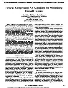
The main idea behind Step 2 in Algorithm 1 is that a new cluster is added to preexisting ones. In [21] an improvement for the h-means algorithm, j-means, is given, to avoid so-called degenerated solutions, where one cluster is empty: the furthest point from all cluster centers is taken as a new center. This leads to an interesting idea, however it needs to be further improved: often real-world datasets contain erroneous records which can be quite far from the rest of the dataset. Taking such an erroneous point as an initial guess may lead to a shallow local minimum. In Figure 1, the point P1 is the furthest point from the cluster centers. However if this point is chosen as the center of a cluster, this cluster will consist of only P1 . The point P2 is closer to the centers, however it would induce a much better cluster. The following algorithm allows one to avoid this difficulty. Algorithm 2 An algorithm for finding the initial point in problem (5). Step 1. (Initialization). Let C1 , . . . , Cq−1 , q ≥ 2 be the preexisting centers and ρ > 0 a tolerance. Let A1 = A, and i = 1. Step 2. Let C be the point in Ai the furthest from the centers C1 , . . . , Cq−1 . Step 3. Find the set �
�
C = a ∈ Ai : kC − ak
ρ, then Cq = C and the algorithm terminates. Otherwise go to Step 4. Step 4. Set Ai+1 = Ai \ {C}, i = i + 1, and go to Step 2. 6
P1
Figure 1: An example of a dataset containing an erroneous point Remark 1 Since A contains a finite number of points the initial guess will be found after a finite number of steps. If the tolerance ρ is too small then the initial guess may be an erroneous point, but if ρ is large then no initial point can be found. Results of numerical experiments show that the tolerance ρ should be chosen in h i m 0.1 m , 0.4 . q q
4
Solving optimization problems
Both problems (3) and (5) in the clustering algorithm are nonsmooth optimization problems. Since the objective functions in these problems are represented as a sum of minimum of norms they are Lipschitz continuous. In order to describe differential properties of the objective functions f and f¯ we recall some definitions from nonsmooth analysis (see [13, 15]).
4.1
Differential properties of the objective functions
We consider a locally Lipschitz function ϕ defined on IRn . This function is differentiable almost everywhere and one can define for it a Clarke subdifferential (see [13]), by �
∂ϕ(x) = co
�
v ∈ IRn : ∃(xk ∈ D(ϕ), xk → x, k → +∞) : v = lim ∇ϕ(xk ) , k→+∞
here D(ϕ) denotes the set where ϕ is differentiable, co denotes the convex hull of a set. The function ϕ is differentiable at the point x ∈ IRn with respect to the direction g ∈ IRn if the limit ϕ(x + αg) − ϕ(x) ϕ0 (x, g) = lim α→+0 α 7
exists. The number ϕ0 (x, g) is said to be the derivative of the function ϕ with respect to the direction g ∈ IRn at the point x. The upper derivative ϕ0 (x, g) of the function ϕ at the point x with respect to the direction g ∈ IRn is defined as follows: ϕ(y + αg) − ϕ(y) . α α→+0,y→x
ϕ0 (x, g) = lim sup The following is true (see [13])
ϕ0 (x, g) = max {hv, gi : v ∈ ∂ϕ(x)} where h·, ·i stands for the inner product in IRn . It should be noted that the upper derivative always exists for locally Lipschitz functions. The function ϕ is said to be regular at the point x ∈ IRn if ϕ0 (x, g) = ϕ0 (x, g) for all g ∈ IRn . For regular functions there exists a calculus (see [13, 15]). However in general for non-regular functions such a calculus does not exist. The function ϕ is called semismooth at x ∈ IRn , if it is locally Lipschitz continuous at x and for every g ∈ IRn , the limit lim
v∈∂ϕ(x+tg 0 ),g 0 →g,t→+0
hv, gi
exists (see [32]). Since both functions f from (4) and f¯ from (6) are locally Lipschitz continuous they are subdifferentiable. Proposition 1 The functions f and f¯ are semismooth. Proof: The sum and the minimum of semismooth functions are semismooth (see [32]). A norm as a convex function is semismooth. Then the function f which is the sum of functions represented as the minimum of norms is semismooth. Similarly the function f¯ which is the sum of functions represented as the minimum of constants and a norm is semismooth as well. 4 Functions represented as a minimum of norms in general are not regular. Since the sum of non-regular functions in general is not regular, the functions f and f¯ in general are not regular. Therefore, subgradients of these functions cannot be calculated using subgradients of their terms. We can conclude that the calculation of the subgradients of the functions f and f¯ is a very difficult task and therefore the application of methods of nonsmooth optimization requiring a subgradient evaluation at each iteration, including bundle method and its variations ([24, 28, 31]), cannot be effective to solve problems (3) and (5). The problems (3) and (5) are global optimization problems. However, they have to be solved many times in Algorithm 1, and thus require fast algorithms. Moreover 8
the number of variables in the problem (3) is large and the global optimization methods cannot be directly applied to solve it. Therefore we will discuss algorithms for finding local minima of the functions f and f¯. Since the evaluation of subgradients of the function f is difficult, direct search methods of optimization seem to be the best option for solving problems (3) and (5). Among such methods we mention here two widely used methods: Powell’s method (see [35]) which is based on a quadratic interpolation of the objective function and Nelder-Mead’s simplex method [34]. Both methods perform well for smooth functions. Moreover they are only effective when the number of variables is less than 20. However, in both problems (3) and (5) the objective functions are quite complicated nonsmooth functions. In the problem (3) the number of variables is nv = n × q where n is the dimension of the dataset A (ranging from 2 to thousands in real world datasets), and q is the number of clusters. In many cases the number nv is greater than 20. In this paper we use the discrete gradient method to solve the problems (3) and (5). The description of this method can be found in [4] (see, also, [5, 6]). The discrete gradient method can be considered as a version of the bundle method ([24, 28, 31]), where subgradients of the objective function are replaced by its discrete gradients. The discrete gradient method uses only values of the objective function. It should be noted that the calculation of the objective functions in the problems (3) and (5) can be expensive as the number of instances in the dataset grows. We will show that the use of the discrete gradient method allows one to significantly reduce the number of objective function evaluations.
4.2
Discrete gradient method
In this subsection we will briefly describe the discrete gradient method. We start with the definition of the discrete gradient. 4.2.1
Definition of the discrete gradient
Let ϕ be a locally Lipschitz continuous function defined on IRn . Let S1 = {g ∈ IRn : kgk = 1}, G = {e ∈ IRn : e = (e1 , . . . , en ), |ej | = 1, j = 1, . . . , n}, P = {z(λ) : z(λ) ∈ IR1 , z(λ) > 0, λ > 0, λ−1 z(λ) → 0, λ → 0}, I(g, α) = {i ∈ {1, . . . , n} : |gi | ≥ α}, where α ∈ (0, n−1/2 ] is a fixed number. Here S1 is the unit sphere, G is the set of vertices of the unit hypercube in IRn and P is the set of univariate positive infinitesimal functions. We define operators Hij : IRn → IRn for i = 1, . . . , n, j = 0, . . . , n by the formula Hij g =
�
(g1 , . . . , gj , 0, . . . , 0) (g1 , . . . , gi−1 , 0, gi+1 , . . . , gj , 0, . . . , 0) 9
if j < i, if j ≥ i.
(7)
We can see that Hij g
−
Hij−1 g
�
=
if j = 1, . . . , n, j 6= i, if j = i.
(0, . . . , 0, gj , 0, . . . , 0) 0
(8)
Let e(β) = (βe1 , β 2 e2 , . . . , β n en ), where β ∈ (0, 1]. For x ∈ IRn we consider vectors xji ≡ xji (g, e, z, λ, β) = x + λg − z(λ)Hij e(β), (9) where g ∈ S1 , e ∈ G, i ∈ I(g, α), z ∈ P, λ > 0, j = 0, . . . , n, j 6= i. It follows from (8) that xj−1 i
−
xji
�
=
(0, . . . , 0, z(λ)ej (β), 0, . . . , 0) 0
if j = 1, . . . , n, j 6= i, if j = i.
(10)
It is clear that Hi0 g = 0 and x0i (g, e, z, λ, β) = x + λg for all i ∈ I(g, α). Definition 1 (see [3, 6]) The discrete gradient of the function ϕ at the point x ∈ IRn is the vector Γi (x, g, e, z, λ, β) = (Γi1 , . . . , Γin ) ∈ IRn , g ∈ S1 , i ∈ I(g, α), with the following coordinates: i
h
Γij = [z(λ)ej (β)]−1 ϕ(xij−1 (g, e, z, λ, β)) − ϕ(xji (g, e, z, λ, β)) , j = 1, . . . , n, j 6= i,
Γii = (λgi )−1 ϕ(xni (g, e, z, λ, β)) − ϕ(x) −
n X
Γij (λgj − z(λ)ej (β)) .
j=1,j6=i
A more detailed description of the discrete gradient and examples can be found in [4, 6]. Remark 2 It follows from Definition 1 that for the calculation of the discrete gradient Γi (x, g, e, z, λ, β), i ∈ I(g, α) we define a sequence of points i+1 n x0i , . . . , xi−1 i , xi , . . . , xi .
For the calculation of the discrete gradient it is sufficient to evaluate the function ϕ at each point of this sequence. Remark 3 The discrete gradient is defined with respect to a given direction g ∈ S1 . We can see that for the calculation of one discrete gradient we have to calculate (n+1) n values of the function ϕ: at the point x and at the points x0i , . . . , xii−1 , xi+1 i , . . . , xi , i ∈ I(g, α). For the calculation of another discrete gradient at the same point with respect to another direction g 1 ∈ S1 we have to calculate this function n times, because we have already calculated ϕ at the point x.
10
4.2.2
Calculation of the discrete gradients of the objective function (4)
Now let us return to the objective function f of the problem (3). This function depends on n × q variables where q is the number of clusters. This function is represented as a sum of min-type functions f (x) =
m X
ψi (x)
i=1
where ψi (x) = min [ηij (x)]θ , i = 1, . . . , m j=1,...,q
with θ =
γ p,
and ηij (x) =
n X
|xju − aiu |p .
u=1
It should be noted that the functions ηij are separable. We can see that for every i = 1, . . . , m, each variable xj appears in only one function ηij . For a given k = 1, . . . , nq we set �
rk =
k−1 + 1, dk = k − (rk − 1)n n �
where bcc stands for the floor of a number c. We define by X the vector of all variables xj , j = 1, . . . , q: X = (X1 , X2 , . . . , Xnq ) where Xk = xrdkk . We use the vector of variables X to define a sequence Xt0 , . . . , Xtt−1 , Xtt+1 , . . . , Xtnq , t ∈ I(g, α), g ∈ IRnq as in Remark 2. It follows from (10) that the points Xtk−1 and Xtk differ by one coordinate only (k = 0, . . . , nq, k 6= t). For every i = 1, . . . , m this coordinate appears in only one function ηirk . It follows from the definition of the operator H that Xtt = Xtt−1 and thus this observation is also true for Xtt+1 . Then we get ηij (Xtk ) = ηij (Xtk−1 ) ∀j 6= rk which means that when we change the k-th coordinate of the point X only one function (namely the function ηirk ) changes its value. Moreover the function ηirk can be calculated at the point Xtk using the value of this function at the point Xtk−1 , k ≥ 1: ηirk (Xtk ) = ηirk (Xtk−1 ) + |xrdkk + z(λ)ek (β) − aidk |p − |xrdkk − aidk |p .
11
(11)
Because η is separable, only one term in the sum changes. Thus we need to add the new term, and subtract the old one. For p = 2 (11) can be simplified as follows �
�
ηirk (Xtk ) = ηirk (Xtk−1 ) + z(λ)ek (β) 2xrdkk + z(λ)ek (β) − 2aidk . In order to calculate the function f at the point Xtk , k ≥ 1 first we have to calculate the values of the functions ηirk for all ai ∈ A, i = 1, . . . , m using (11). Then we update f using these values and the values of all other functions ηij , j 6= rk at the point Xtk−1 according to (4). Thus we have to apply a full calculation of the function f using the formula(4) only at the point Xt0 = X + λg. Hence for the calculation of each discrete gradient we have to apply a full calculation of the objective function f only at the point Xt0 = X + λg and this function can be updated at the points Xtk , k ≥ 1 using a simplified scheme. We can conclude that for the calculation of the discrete gradient at a point X with respect to the direction g 0 ∈ S1 we calculate the function f at two points: X and Xt0 = X + λg 0 . For the calculation of another discrete gradient at the same point X with respect to another direction g 1 ∈ S1 we calculate the function f only at the point: X + λg 1 . The function f¯(x) ≡ f¯u (x) defined by (6) can be rewritten as follows: f¯(x) =
m X
n
min ci , [¯ ηi (x)]θ
o
i=1
where
n
ci = min kx1∗ − ai kγp , . . . , kxu∗ − ai kγp and η¯i (x) =
n X
o
|xl − ail |p , x ∈ IRn .
l=1
Here θ > 0 is defined as above. The functions η¯i are separable and have a similar structure as the functions ηij . Therefore we can apply a simplified scheme for their calculation as well. Hence we can accelerate the calculation of each discrete gradient of the function f¯ in a similar way as we do for the function f (see above). Since the number of variables nq in the problem (3) can be large this algorithm allows one to significantly reduce the number of objective function evaluations during the calculation of a discrete gradient. Although the number of variables n in the problem (5) is significantly less than in the problem (3) this algorithm still allows one to accelerate the calculation of the discrete gradients of the objective function. 4.2.3
The method
We consider the following unconstrained minimization problem: minimize ϕ(x) subject to x ∈ IRn
12
(12)
where the function ϕ is assumed to be semismooth. An important step in the discrete gradient method is the calculation of a descent direction of the objective function ϕ. Therefore, we first describe an algorithm for the computation of this direction. Let z ∈ P, λ > 0, β ∈ (0, 1], the number c ∈ (0, 1) and a tolerance δ > 0 be given. Algorithm 3 An algorithm for the computation of the descent direction. Step 1. Choose any g 1 ∈ S1 , e ∈ G, i ∈ I(g 1 , α) and compute a discrete gradient v 1 = Γi (x, g 1 , e, z, λ, β). Set D1 (x) = {v 1 } and k = 1. Step 2. Calculate the vector kwk k = min{kwk : w ∈ Dk (x)}. If kwk k ≤ δ,
(13)
then stop. Otherwise go to Step 3. Step 3. Calculate the search direction by g k+1 = −kwk k−1 wk . Step 4. If ϕ(x + λg k+1 ) − ϕ(x) ≤ −cλkwk k,
(14)
then stop. Otherwise go to Step 5. Step 5. Calculate a discrete gradient v k+1 = Γi (x, g k+1 , e, z, λ, β), i ∈ I(g k+1 , α), construct the set Dk+1 (x) = co {Dk (x) {v k+1 }}, set k = k + 1 and go to Step 2. S
We give some explanations to Algorithm 3. In Step 1 we calculate the first discrete gradient with respect to an initial direction g 1 ∈ IRn . The distance between the convex hull Dk of all calculated discrete gradients and the origin is calculated in Step 2. This problem can be solved using Wolfe’s algorithm ([41]). If this distance is less than the tolerance δ > 0 then we accept the point x as an approximate stationary point (Step 2), otherwise we calculate another search direction in Step 3. In Step 4 we check whether this direction is a descent direction. If it is we stop and the descent direction has been calculated, otherwise we calculate another discrete gradient with respect to this direction in Step 5 and update the set Dk . At each iteration k we improve the approximation Dk of the subdifferential of the function ϕ. It is proved that Algorithm 3 is terminating (see [4]). Now we can describe the discrete gradient method. Let sequences δk > 0, zk ∈ P, λk > 0, βk ∈ (0, 1], δk → +0, zk → +0, λk → +0, βk → +0, k → +∞ and numbers c1 ∈ (0, 1), c2 ∈ (0, c1 ] be given.
13
Algorithm 4 Discrete gradient method Step 1. Choose any starting point x0 ∈ IRn and set k = 0. Step 2. Set s = 0 and xks = xk . Step 3. Apply Algorithm 3 for the calculation of the descent direction at x = xks , δ = δk , z = zk , λ = λk , β = βk , c = c1 . This algorithm terminates after a finite number of iterations l > 0. As a result we get the set Dl (xks ) and an element vsk such that kvsk k = min{kvk : v ∈ Dl (xks )}. Furthermore either kvsk k ≤ δk or for the search direction gsk = −kvsk k−1 vsk ϕ(xks + λk gsk ) − ϕ(xks ) ≤ −c1 λk kvsk k.
(15)
kvsk k ≤ δk
(16)
Step 4. If then set xk+1 = xks , k = k + 1 and go to Step 2. Otherwise go to Step 5. Step 5. Construct the following iteration xks+1 = xks + σs gsk , where σs is defined as follows n o σs = arg max σ ≥ 0 : ϕ(xks + σgsk ) − ϕ(xks ) ≤ −c2 σkvsk k . Step 6. Set s = s + 1 and go to Step 3. For the point x0 ∈ IRn we consider the set M (x0 ) = {x ∈ IRn : ϕ(x) ≤ ϕ(x0 )}. Theorem 1 Assume that the set M (x0 ) is bounded for starting points x0 ∈ IRn . Then every accumulation point of {xk } belongs to the set X 0 = {x ∈ IRn : 0 ∈ ∂ϕ(x)}. Since the objective functions in problems (3) and (5) are semismooth the discrete gradient method can be applied to solve them. Discrete gradients in Step 5 of Algorithm 3 can be calculated using the simplified schemes described above.
5
Results of numerical experiments
To verify the effectiveness of the proposed approach a number of numerical experiments with real-world data sets have been carried out on a Pentium-4, 1.7 GHz, PC. The following datasets have been used in numerical experiments: 1. Fisher’s iris dataset (m = 150, n = 4) [18]; 2. Image segmentation dataset (m = 2310, n = 19) [33]; 3. The traveling salesman problem - TSPLIB1060 (m = 1060, n = 2) [37]; 14
4. The traveling salesman problem - TSPLIB3038 (m = 3038, n = 2) [37]. In order to implement Algorithm 4 we have to select the sequences {δk }, δk > 0, {zk }, zk ∈ P, {λk }, λk > 0, {βk }, βk ∈ (0, 1]. In the numerical experiments we chose these sequences as follows: δk = 10−9 , βk = 1 for all k, zk (λ) = λα , α ∈ [1.5, 4], λk = dk λ0 , d = 0.5, λ0 = 0.9. We take λmin ∈ (0, λ0 ). If λk < λmin then Algorithm 4 terminates. In order to get a solution with high accuracy one has to take λmin very small, for example λmin ≤ 10−5 . Larger values of λmin may lead to more inaccurate solutions, however Algorithm 4 calculates such solutions very quickly. In our numerical experiments, unless specified otherwise, we set λmin large. In the numerical experiments we also take c1 = 0.2 and c2 = 0.001. The starting point for solving problem (5) is generated by Algorithm 2 and the starting point for solving problem (3) is generated in Algorithm 1. In Algorithm 2 we fix the parameter ρ = rm q where r ∈ [0, 0.5]. For image segmentation dataset we take λmin = 10−5 . For all other datasets this parameter is: λmin = 0.01. In the numerical experiments we consider the squared Euclidean norm, that is γ = 2 and p = 2. In order to provide comparison with the best known solutions from the literature we calculated 10 clusters for iris dataset and 50 clusters for all other datasets. Algorithm 1 is a deterministic one. However, it requires the selection of the parameter ρ, which determines the starting points. To see how this parameter influences the results, numerical experiments have been carried out for ri = 0.05i, i = 0, . . . , 10. We present the results of the numerical experiments in Tables 1-4. In these tables k represents the number of clusters. We give the best known function value fopt from the literature corresponding to k clusters ([21, 23]) and the % error Ebest and Emean of respectively the best value and the average value obtained by the proposed algorithm. The error E is calculated as E=
(f¯ − fopt ) · 100 fopt
where f¯ is the function value obtained by the algorithm. A negative error means that the proposed algorithm improved the best known solution. We also give the average number of calculations of norms for reaching the solutions. Ns and Ng represent the average number of norm evaluations for finding k clusters using the simplified and general schemes, respectively. In the tables we give the values of Ns and the ratio Ng /Ns . Finally, in these tables we present the average CPU time (t) and its standard deviation (σt ). Results presented in Tables 1-4 show that for Fisher’s iris, TSPLIB3038 and TSPLIB1060 datasets the proposed algorithm allows one to calculate either the best known solution or a solution which is very close to the best one. For image segmentation dataset the results for large numbers of clusters are not so good which can be explained by the existence of erroneous points. These results demonstrate 15
k 2 3 4 5 6 7 8 9 10
fopt 152.348 78.851 57.226 46.446 39.040 34.298 29.989 27.786 25.834
Ebest 0.00 0.00 0.00 0.00 0.00 0.00 0.00 0.00 0.52
Emean 0.00 0.00 0.00 0.68 0.00 0.86 0.11 2.11 1.78
Ns 1.43 · 105 3.22 · 105 5.83 · 105 8.73 · 105 1.21 · 106 1.57 · 106 2.03 · 106 2.46 · 106 3.00 · 106
Ng /Ns 3.63 5.00 5.95 7.33 8.23 9.31 10.62 11.86 13.04
t 0.10 0.20 0.34 0.49 0.65 0.82 1.04 1.23 1.47
σt 0.02 0.03 0.05 0.05 0.04 0.05 0.07 0.09 0.07
Table 1: Results for Fisher’s Iris dataset that if the algorithm gets stuck in a shallow minimum then it may affect the next iterations. However, results for this dataset show that the algorithm in most cases reaches a solution which is close to the best one. It should be noted that the problem of finding 50 clusters in the image segmentation dataset has 950 variables which is challenging for many global optimization techniques. The results for the error of average values presented in these tables show that for Fisher’s iris, TSPLIB3038 and TSPLIB1060 datasets the results obtained by the proposed algorithm do not strongly depend on the initial point (that is values of ρ) and they are always close to the best solutions. The results for the image segmentation dataset are more dependent on the initial point. This is an indicator of the existence of erroneous points in this dataset. This shows that if a dataset does not have a good cluster structure the proposed algorithm may lead to different solutions starting from different initial points. The results for the number Ns show that one can calculate a large number of clusters using a reasonable number of norm evaluations. The ratio Ng /Ns demonstrate that the simplified scheme allows one to significantly reduce the computational effort. This complexity reduction becomes larger as the number of clusters or the number of features increase. The results presented in the tables show that the clustering problem can be solved by the algorithm within reasonable CPU time. CPU time depends on the parameter λmin . Small values of λmin lead to a better solution, however much more CPU time is required as in the case of the image segmentation dataset. The result for σt show that the CPU time does almost not depend on starting points.
6
Conclusions
In this paper we have formulated the clustering problem as a nonsmooth nonconvex optimization problem and proposed a clustering algorithm based on nonsmooth optimization techniques. The discrete gradient method has been used for solving the nonsmooth optimization problems. We have adapted this method to this problem
16
k 2 3 4 5 6 7 8 9 10 20 30 40 50
fopt 3.5606 · 107 2.7416 · 107 1.9456 · 107 1.7143 · 107 1.5209 · 107 1.3404 · 107 1.2030 · 107 1.0784 · 107 9.7952 · 106 5.1283 · 106 3.5076 · 106 2.7398 · 106 2.2248 · 106
Ebest -0.01 -0.02 -0.03 -0.03 -0.03 0.33 2.28 1.36 1.51 -0.01 5.62 9.96 15.26
Emean 2.08 4.90 15.82 13.16 16.36 10.50 14.29 9.28 8.72 8.76 10.21 13.52 19.30
Ns 8.14 · 106 1.86 · 107 3.60 · 107 5.45 · 107 7.73 · 107 1.04 · 108 1.30 · 108 1.61 · 108 1.90 · 108 2.48 · 108 3.33 · 108 3.50 · 108 3.65 · 108
Ng /Ns 20.69 27.31 33.70 40.41 47.34 54.77 62.96 70.12 77.12 111.15 184.89 207.80 231.72
t 19.43 40.05 69.37 98.53 131.88 169.15 205.52 248.53 289.24 897.46 1815.14 2396.03 3011.10
σt 3.12 6.93 12.92 22.23 32.67 47.53 49.40 70.28 74.52 198.27 255.73 247.34 241.75
Table 2: Image Segmentation dataset
k 2 3 4 5 6 7 8 9 10 20 30 40 50
fopt 3.1688 · 109 2.1763 · 109 1.4790 · 109 1.1982 · 109 9.6918 · 108 8.3966 · 108 7.3475 · 108 6.4477 · 108 5.6025 · 108 2.6681 · 108 1.7557 · 108 1.2548 · 108 9.8400 · 107
Ebest 0.00 0.00 0.00 0.00 0.00 1.73 0.00 0.00 0.00 0.00 0.27 -0.08 0.62
Emean 0.00 1.51 0.03 0.21 0.05 1.91 0.75 0.44 0.68 0.90 1.55 1.48 1.63
Ns 1.78 · 106 4.31 · 106 6.62 · 106 9.56 · 106 1.26 · 107 1.52 · 107 1.94 · 107 2.34 · 107 2.78 · 107 3.40 · 107 4.32 · 107 5.45 · 107 6.82 · 107
Ng /Ns 1.69 2.24 2.82 3.35 3.90 4.54 5.20 5.94 6.73 10.07 16.56 24.70 33.88
t 0.74 1.65 2.48 3.50 4.56 5.53 6.99 8.41 9.98 29.35 61.04 104.74 158.03
σt 0.17 0.19 0.14 0.16 0.16 0.11 0.32 0.40 0.37 1.04 1.35 1.72 3.83
t 4.61 13.62 29.02 81.90
σt 0.42 1.08 1.48 3.72
Table 3: TSPLIB3038 dataset
k 10 20 30 50
fopt 1.75484 · 109 7.91794 · 109 4.81251 · 109 2.55509 · 109
Ebest 0.00 0.32 1.29 1.36
Emean 0.18 3.01 3.76 2.46
Ns 1.39 · 107 1.77 · 107 2.46 · 107 4.48 · 107
Ng /Ns 6.00 8.74 14.03 28.12
Table 4: TSPLIB1060 Dataset
17
which allows one to considerably accelerate its convergence. The clustering algorithm calculates clusters incrementally. This algorithm calculates as many clusters as a dataset contains with respect to some tolerance. The proposed algorithm has been tested using real-world datasets. The results of these experiments demonstrate that the algorithm can calculate a satisfactory solution within a reasonable CPU time. These results explicitly show that the algorithm allows one to significantly reduce the computational effort which is extremely important for clustering in large scale data sets. Acknowledgements This research was supported by the Australian Research Council.
References [1] K.S. Al-Sultan, A tabu search approach to the clustering problem, Pattern Recognition, 28(9), 1995, 1443-1451. [2] K.S. Al-Sultan and M.M. Khan, Computational experience on four algorithms for the hard clustering problem, Pattern Recognition Letters, 17, 1996, 295-308. [3] A.M. Bagirov and A.A. Gasanov, A method of approximating a quasidifferential, Russian Journal of Computational Mathematics and Mathematical Physics, 35(4), 1995, 403-409. [4] A.M. Bagirov, Minimization methods for one class of nonsmooth functions and calculation of semi-equilibrium prices, In: A. Eberhard et al. (eds.) Progress in Optimization: Contribution from Australasia, Kluwer Academic Publishers, 1999, 147-175. [5] A.M. Bagirov, A method for minimzation of quasidifferentiable functions, Optimization Methods and Software, 17(1), 2002, 31-60. [6] A.M. Bagirov, Continuous subdifferential approximations and their applications, Journal of Mathematical Sciences, 115(5), 2003, 2567-2609. [7] A.M. Bagirov, A.M. Rubinov and J. Yearwood, A global optimisation approach to classification, Optimization and Engineering, 3(2), 2002, 129-155. [8] A.M. Bagirov, A.M. Rubinov, N.V. Soukhoroukova and J. Yearwood, Supervised and unsupervised data classification via nonsmooth and global optimisation, TOP: Spanish Operations Research Journal, 11(1), 2003, 1-93. [9] A.M. Bagirov and J. Yearwood, A new nonsmooth optimization algorithm for minimum sum-of-squares clustering algorithms, European Journal Operational Research, to appear.
18
[10] H.H. Bock, Automatische Klassifikation, Vandenhoeck & Ruprecht, Gottingen, 1974. [11] H.H. Bock, Clustering and neural networks, In: A.Rizzi, M. Vichi and H.H. Bock (eds), Advances in Data Science and Classification, Springer-Verlag, Berlin, 1998, 265-277. [12] D.E. Brown and C.L. Entail, A practical application of simulated annealing to the clustering problem, Pattern Recognition, 25, 1992, 401-412. [13] F.H. Clarke, Optimization and Nonsmooth Analysis, Wiley, New York, 1983. [14] O. du Merle, P. Hansen, B. Jaumard and N. Mladenovic, An interior point method for minimum sum-of-squares clustering, SIAM J. on Scientific Computing, 21, 2001, 1485-1505. [15] V.F. Demyanov and A.M. Rubinov, Constructive Nonsmooth Analysis, Peter Lang, Frankfurt am Main, 1995. [16] G. Diehr, Evaluation of a branch and bound algorithm for clustering, SIAM J. Scientific and Statistical Computing, 6, 1985, 268-284. [17] R. Dubes and A.K. Jain, Clustering techniques: the user’s dilemma, Pattern Recognition, 8, 1976, 247-260. [18] R.A. Fisher, The use of multiple measurements in taxonomic problems, Ann. Eugenics, VII part II (1936), 179-188. Reprinted in R.A. Fisher, Contributions to Mathematical Statistics, Wiley, 1950. [19] P. Hanjoul and D. Peeters, A comparison of two dual-based procedures for solving the p-median problem, European Journal of Operational Research, 20, 1985, 387-396. [20] P. Hansen and B. Jaumard, Cluster analysis and mathematical programming, Mathematical Programming, 79(1-3), 1997, 191-215. [21] P. Hansen and N. Mladenovic, J-means: a new heuristic for minimum sum-ofsquares clustering, Pattern Recognition, 4, 2001, 405-413. [22] P. Hansen and N. Mladenovic, Variable neighborhood decomposition search, Journal of Heuristic, 7, (2001), 335-350. [23] P. Hansen, E. Ngai, B.K. Cheung and N. Mladenovic, Analysis of global kmeans, an incremental heuristic for minimum sum-of-squares clustering, submitted [24] J.-P. Hiriart-Urruty and C. Lemarechal, Convex Analysis and Minimization Algorithms, Vol. 1 and 2, Springer-Verlag, Berlin, New York, 1993.
19
[25] D.M. Houkins, M.W. Muller and J.A. ten Krooden, Cluster analysis, In: Topics in Applied Multivariate Analysis, Cambridge University press, Cambridge, 1982. [26] A.K. Jain, M.N. Murty and P.J. Flynn, Data clustering: a review, ACM Computing Surveys 31(3), 1999, 264-323. [27] R.E. Jensen, A dynamic programming algorithm for cluster analysis, Operations Research, 17, 1969, 1034-1057. [28] K.C. Kiwiel, Methods of descent for nondifferentiable optimization, Lecture Notes in Mathematics, 1133, Springer-Verlag, Berlin, 1985. [29] W.L.G. Koontz, P.M. Narendra and K. Fukunaga, A branch and bound clustering algorithm, IEEE Transactions on Computers, 24, 1975, 908-915. [30] A. Likas, M. Vlassis and J. Verbeek, The global k-means clustering algorithm, Pattern Recognition, 36, 2003, 451-461. [31] M.M. Makela and P. Neittaanmaki, Nonsmooth Optimization, World Scientific, Singapore, 1992. [32] R. Mifflin, Semismooth and semiconvex functions in constrained optimization, SIAM Journal on Control and Optimization, 15(6), 1977, 959-972. [33] P.M. Murphy and D.W. Aha, UCI repository of machine learning databases, Technical report, Department of Information and Computer Science, University of California, Irvine, 1992, www.ics.uci.edu/mlearn/MLRepository.html. [34] J.A. Nelder and R. Mead, A simplex method for function minimization, Comput. J., 7, 1965, 308-313. [35] M.J.D. Powell, UOBYQA: unconstrained optimization by quadratic approximation, Mathematical Programming, Series B, 92(3), 2002, 555-582. [36] C.R. Reeves (ed.), Modern Heuristic Techniques for Combinatorial Problems, Blackwell, London, 1993. [37] G. Reinelt, TSP-LIB-A Traveling Salesman Library, ORSA J. Comput. 3, 1991, 319-350. [38] S.Z. Selim and K.S. Al-Sultan, A simulated annealing algorithm for the clustering, Pattern Recognition, 24(10), 1991, 1003-1008. [39] H. Spath, Cluster Analysis Algorithms, Ellis Horwood Limited, Chichester, 1980. [40] L.X. Sun, Y.L. Xie, X.H. Song, J.H. Wang and R.Q. Yu, Cluster analysis by simulated annealing, Computers and Chemistry, 18, 1994, 103-108. 20
[41] Wolfe, P.H., Finding the nearest point in a polytope, Mathematical Programming, 11(2), 1976, 128-149.
21