JOURNAL OF COMPUTERS, VOL. 6, NO. 8, AUGUST 2011
1781
An Algorithm for Minimum Vertex Cover Based on Max-I Share Degree Shaohua Li1,2 1
Department of Computer Science & Technology,Guangdong University of Business Studies,Guangzhou 510320,China Email:
[email protected]
Jianxin Wang 2, Jianer Chen2,3 and Zhijian Wang1 2 3
School of Information Science and Engineering of Central South University, Changsha 410083, China Department of Computer Science of Texas A&M University, College Station, Texas 77843-3112, USA Email: {
[email protected],
[email protected],
[email protected] }
Abstract—Minimum vertex cover problem(Min-VC) on a graph is a NP-hard problem. The neighborhoods of a vertex are analyzed in this paper, and so are the information they hold for judging whether the vertex is belong to Min-VC or not. Then, the concept of Max-I share degree is put forword in order to qualify the possibility of a vertex to be collected into Min-VC. Based on Max-I share degree, a heuristic algorithm is proposed. Our algorithm has two remarkable characteristics: one is that it is able to get almost the same Min-VC as that of an exact algorithm, and the approximation degree is obviously better than that of other approximation algorithms; the other is that it has polynomial time complexity. Emulational results show that the running time is significantly less than those of other algorithms. Index Terms—vertex cover, share degree, approximation degree, heuristic algorithm
I. INTRODUCTION Given a graph G = (V, E), a minimum vertex cover problem (Min-VC) of the graph G is a subset V′ of vertices such that for every edge (u, v)∈E, at least one of u, v belongs to this subset V′. Min-VC problem is one of Karp′s 21 NP-complete problems [1], and is therefore a classical NP-complete problem in computational complexity theory [2]. Min-VC can be reduced to maximum clique problem and maximum independent set problem, it has widely applications in many fields, such as network security, sensor networks, scheduling, VLSI design and bioinformatics [3], etc. For example, accurate network flow measurement is important for a variety of network applications, where the "flow" over an edge in the network is intuitively the rate of data traffic. The problem of efficiently monitoring the network flow can be regarded as finding the minimum weight weak vertex cover for a given graph. Since the complexity of Min-VC has been heavily studied since Karp’s original proof of its NPSupported by the National Basic Research 973 Program of China No.2008CB317107, the National Natural Science Foundation of China Nos.60433020, 60773111 and the Natural Science Foundation of Guangdong Province No. 8451032001001610.
© 2011 ACADEMY PUBLISHER doi:10.4304/jcp.6.8.1781-1788
completeness, the related bibliography is vast and cannot be covered, of course, in this introductory note. Research on Min-VC has mainly three ways. The one is to design an exact algorithm. According to the NP-completeness theory, Min-VC cannot be solved in polynomial time unless P = NP, which means it is unlikely that there is an efficient algorithm to solve it exactly. Vertex cover remains NP-complete even in cubic graphs [4] and even in planar graphs of degree at most 3 [5]. The second landscape for exact algorithm design of vertex cover problem is parameterized complexity theory[6,7], which is committed to design fixed-parameter tractability algorithms for NP-complete problems. Parameterized complexity has nowadays become a standard way of dealing with NP-hard problems. Parameterized vertex cover problem is defined as bellow: K-Vertex Cover Problem: Input: A graph G and a positive integer k; Parameter: k; Question:Does G have a vertex cover with at most k vertices? A parameterized problem Q is kernelizable if there exists a polynomial time algorithm A (the "kernelization algorithm") and a recursive function g such that any instance (x, k) of Q, the algorithm A produces an instance (x′,k′) of Q (the "kernel"), such that |x′|≤g(k) and k′≤k, and that (x, k) is a yes-instance of Q if and only if (x′,k′) is a yes-instance of Q. Chen J. et.al[8] proposed a kernelization algorithm for K-Vertex Cover Problem. In [8], several reduction rules were proposed, and then applied crown decomposition technique to further reduce the graph, which lead to an exact algorithm of time O(kn + 1.2852k) for K-Vertex Cover Problem. However, if we want to find a minimum vertex cover of graph G, parameter k doesn’t exist anymore. The third way is to find a near-optimal solution in polynomial time. An algorithm that runs in polynomial time and outputs a solution close to the optimal solution is called an approximation algorithm. Min-VC is known to be APXcomplete [9], and moreover it cannot be approximated within a factor of 1.36 [10], unless P = NP. Heuristic method is a widely used and effective method for approximation algorithm design. Current heuristic algorithms of Min-VC only consider vertex features in
1782
JOURNAL OF COMPUTERS, VOL. 6, NO. 8, AUGUST 2011
isolation in order to decide whether the vertex in or not in the solution set, greedy-edge algorithm and greedydegree algorithm [11,12], for example. But by observation, not only should we consider its topological properties of a vertex, but also the local structure of the graph. In our opinion, the solution set of Min-VC mainly relies on the complex relationship between vertices. It is a huge waste of computational time if we assess a vertex with global perspective. Furthermore, the global relationship between vertices is affected by their direct or indirect neighborhoods. In one word, the neighborhood relationship of a vertex has its special roles in Min-VC solving process. We propose here a concept of Max-I share degree, and design a heuristic algorithm based on Max-I share degree. We analyze our algorithm from the theoretical and experimental aspects. Theory and experiment show that our algorithm is basically the same results with the exact algorithm, significantly better than other heuristic methods.
I.
CORRELATIONAL RESEARCH
A. Exact Algorithm Design The time complexity of the exact algorithm for solving the minimum vertex cover is generally increased with the graph size (number of vertices n). Because each vertex of a graph is either a covering point or a non-covering point, the most direct way is to enumerate all possible 2n combinations and then to judge which combination is the minimum vertex cover set. Techniques for exact algorithm design of Min-VC are mainly both divide-andconquer method and branch-and-bound method. Divideand-conquer method firstly identifies all the connected components of a graph, and then recursively calculates the minimum vertex cover set of each connected component. The basic idea for handling each connected component is: suppose S(G) is a minimum vertex cover solution set of G and N(u)⊂V is the neighborhoods of u in G. Let G(Vs)=(Vs, E(Vs)) is induced subgraph of Vs⊂V, i.e, E(Vs)=È∩(Vs × Vs), then either S={u}∪S(G(V\{u})) or S={N(u)}∪S(G(V\{u}\N(u))). Furthermore, for some small-scale graph Vs, we can exclude some vertices from consideration in the next step if we can prove that they can not cover the edges between Vs and V\Vs. or produce a better solution set. For example, according to the leafremoval heuristic of Bauer and Golinelli[13], leaf nodes is dominated. Suppose u is a leaf node of vertex v, then u should be in S(G), and v should be excluded. Excluding the dominated vertices makes exact algorithm run faster, but such an algorithm can only returns one solution set. If we want to get all the solution results, branch-and-bound technique is required. B. Approximation Algorithm Design There are many kinds of approximation algorithms for Min-VC. Cormen T. H. et al.[14] proposed a heuristic approximation algorithm AVC which its approximation degree is 2. Its basic ideas are: (1) Randomly selecting a edge e(u, v) from the graph G, and then put its two endpoints u and v into the minimum solution set; (2)deleting the edge e and all the adjacent vertices of u © 2011 ACADEMY PUBLISHER
and v. Yang Jie and Wang Ling [11] designed an approximation algorithm GEAVC based on greedy-edge, which achieved a better solution result than AVC algorithm and its approximation degree is no bigger than two. The kernel ideas are: (1) single vertex greedy edge rule: rule to reduce degree one vertices. (2) double vertex greedy edge rule: rule to reduce degree two vertices. Dinur and Safra[10] proved that the approximation factor of Min-VC could not be better than 1.36, unless P = NP. There are however many natural special-case graph classes for which one can improve on this barrier. For instance, in the class of interval graphs, which can be thought of as one dimensional analog of rectangle graphs, Minimum Vertex Cover is polynomial time solvable [15]. In planar graphs, the problem is known to admit a polynomial-time approximation scheme (PTAS) [16], and even an efficient PTAS (EPTAS) due to Baker’s seminal framework for NP-hard planar graph problems [17]. Karakostas G.[18] designed a generalized heuristic approximation algorithm for Min-VC. The algorithm defined a search depth parameter ρ. For any a vertex u, suppose its probability selected into the covering set is wd(u). The probability depends on u’s current degree d(u). Let G(ρ)(u)=(V(ρ)(u), E(ρ)(u)), where V(ρ)(u) includes all those vertices that the path length to u is no bigger than ρ, E(ρ)(u) consists of edges between vertices of V(ρ)(u). G(ρ)(u) is an induced subgraph of G. If there is a vertex set V' ⊆ V(ρ)(u) that each of which has just ρ path length to u, then V' is selected into the covering set. Next, we pick out the vertex v∈G(ρ)(u)\V' that has the largest path length to u and put v’s neighborhoods(not v) into solution set. Miehalewiez Z. et al.[19] provided an approximation algorithm based on GCEMC(Grand Canonical Ensemble Monte Carlo). Firstly, the algorithm initiates a covering set(for example, let V is a covering set). Secondly, randomly selects a vertex u in each step of GCEMC, and takes a MOVE operation with probability p and an EXCHANGE operation with probability p-1. Unlike other algorithms, [19] allows vertices move into or pop out the covering set, as well as fluctuating of the size of the covering set. [20] gave a faster reduction algorithm which defined a judgement function to analyze its merits of a vertex for minimum vertex cover and further provided a generalization rule for low-degree vertex reduction. [21] presented a hybrid genetic algorithm(HGA) combining SGA and local optimization technique, which improved local searching ability of SGA and gave near to optimal solution speedy. HGA is mainly applied to some special cases. In this paper we focus on the effective Min-VC approximation algorithm of the simple undirected graph. The main contribution of this paper is: We propose a new concept of share degree, and dexterously consider the adjacent vertex influences to minimum vertex cover set, then an approximation algorithm based on Max-I share degree is designed. Emulational results show that our algorithm is more effective and faster than many others.
JOURNAL OF COMPUTERS, VOL. 6, NO. 8, AUGUST 2011
II.
NOTATION AND DEFINITIONS
A graph is defined as a pair G=(V, E), where the elements of V are called vertices of G, V:={v1, . . . , vn}, and the elements of E are called edges, E ⊆ {{u, v} : u, v ∈V }. We denote the set of vertices of a graph G with V(G), and the set of edges E(G). We suppose here that G is a simple graph, i.e, G has no loop and double edges. We use n or |V(G)| to denote the number of vertices and m or |E(G)| to denote the number of edges of a graph G. Two vertices v, w ∈V are called adjacent if there exists an edge {v,w}∈E. The neighborhood N(u) of a vertex u∈V is the set of vertices that are adjacent to u, i.e, N(u)={v|(u, v)∈E}, we also say that u shares N(u) and u is shared by N(u) as well. A vertex v∈V is called incident with an edge e∈ E if v∈e. The degree d(u) of a vertex u is the size |N(u)| of N(u), the number of incident edges. A path P is a graph G= (V, E) with V = {v1, v2, . . . , vn}, E = {{v1, v2}, {v2, v3}, . . . , {vn−1, vn}}, where V is a set of distinct vertices. The two vertices v1 and vn are connected by P. A path connecting two vertices u, v is denoted by Pu,v. The length of a path is defined as the number of its edges. The following gives some definitions and lemmas. Definition 1. Suv denotes the Share degree of u to v, Quv denotes the shared degree of v by u. For a edge e(u ,v)∈E, Suppose v has k neighborhoods, i.e, k=N(v), then u shares k vertices and u is shared by k vertices, so that Suv = Quv = 1/k. Definition 2. Let 1 1 n−1 n−1 1 k x = ∑ x be share degree ρ(x)= x + x 2 + ... + 2 n −1 k =1 k distribution of anyone vertex. Share degree of u to v is actually the possession proportion of N(v). Lemma 1. Suppose 1≤k≤n-1 and 1≤ak≤d(u), let φu(x) = n −1
a1x+ a2x2+..+ an-1xn-1 = ∑ ak x k is the degree distribution k =1
of all the neighborhoods of vertex u. then φu(1)= d(u). n −1
Proof. Because φu(x) =
∑ ak x k , let x=1, then:
k =1
n −1
φu(1) =
1783
∑ ak = d(u)
□
Su a = S ui1 + Sui 2 + ... + Sui a k
k
a k Items 644 744 8 1 1 1 + + ... + k k k
=
= ak
Su= Su1+ Su2+…+ Sud(u) = Sua1 + Su a 2 + ... + Su a 1 2
1 3
= a1 + a2 + a3 + ... +
1 k
, so that:
( n −1)
n −1 1
1 an −1 n −1
= ∑ ak k =1 k
We can also prove lemma 2 according to the relationship between the share degree distribution ρ(x) and the degree distribution of all the neighborhoods of vertex u. i.e, ρu(x) =ρ(x)|x=1 φuT(x) = ρ(1) φuT(x) 1 1 1 )(a1x+ a2 x2+ a3x3 +..+ an-1xn-1)T =( 1 + + + ... + 2 3 n −1 a a a = a1 x + 2 x 2 + 3 x 3 + ... + n−1 x n−1 n −1 2 3 n −1 a = ∑ k xk . k =1 k If we take the distribution variation x into the upper equation, we will have:
ρu(x)= a1x +
n −1 a a a2 2 a3 3 x + x + ... + n −1 x n −1 = ∑ k x k n −1 2 3 k =1 k
□
Definition 3. For u∈V of a general graph G=(V, E), the n −1 a
first i items of ρu(x) = ∑
k =1
k
k
xk
is named I-share degree of
vertex u. Definition 4. For any two vertices u, v∈V of a general n −1 a
graph G=(V,E), let ρu(x)= ∑
k =1
k
k
xk
be the share degree
n −1b k
distribution of vertex u, ρv(x)= ∑
k =1
k
xk
be the share
degree distribution of vertex v. If a1= b1, a2= b2, …, ai-1= bi-1, but ai>bi, then we say that ρu(x)> ρv(x). If ρu(x)≥ρw(x)|w∈V,w≠u, then we say that u is Max-I vertex. Definition 5. Given a graph G and an approximation algorithm A of minimum vertex cover problem, the approximation degree ΘA of algorithm A is defined as ΘA= |C|/|C*|, where C* is the optimal vertex cover set, C is the result set of approximation algorithm A. It is no doubt that 1≤ ΘA≤ n.
k =1
d (u )
Lemma 2. Let Su= Su1+ Su2+…+ Sud(u) =
∑ S ui denote the i =1
sum of the Share degree of u to its d(u) neighborhoods, then the share degree distribution ρu(x) of vertex u is: n −1 a ρu(x) = ∑ k x k . k =1 k Proof. According to Lemma 1, the degree distribution of vertex u’s neighborhoods is: φu(x) =a1x+ a2x2+..+ an-1xn-1. Suppose i1, i2, …, ia k are some neighborhoods of vertex
u, then d(i1)= d(i2)= …=d( ia k )=k. Because φu(x) =a1x+ a2x2+..+ an-1xn-1 and Suv = 1/d(v), then:
© 2011 ACADEMY PUBLISHER
III.
ALGORITHM BASED ON MAX-I SHARE DEGREE
A. Basic Ideas The neighborhoods of a vertex play a very important role in the Min-VC problem. According to this idea, we design a heuristic algorithm based on Max-I share degree. By observation, when we want to decide whether a vertex u is in or not in the minimum vertex cover set C* of a graph G, the following should be considered: we should put such a vertex u into C* that makes the degree of its neighborhoods reduced to zero as much as possible, or makes the total value of the degree decrease of all its neighborhoods as much as possible. It tells us that we should put such a vertex into C* that has Max-I share degree.
1784
JOURNAL OF COMPUTERS, VOL. 6, NO. 8, AUGUST 2011
For example, given a graph(Figure 1). In order to find the minimum vertex cover set C*, the main procedures based on Max-I share degree are as follows. 14 13
3
2
9 8 1 B
7
12
10 15
6 4
11
5 16
Figure 1. An example for algorithm procedures
(1) First, computing the degree distribution of each vertex according to lemma 1. Take vertex 1 for example. Vertex 1 has five neighborhoods. The degree of each of the four vertices 2,3,5,6 is equal to 1, and d(4) =2, so that: φ1(x) = 4x+x2. In similar, we get: φ2(x) =φ3(x) =φ5(x) =φ6(x) = x5 φ7(x) = 5x2 φ8(x) =φ9(x) =φ10(x) =φ11(x) = x + x5 φ4(x)=φ12(x) = x2 + x5 φ13(x) =φ14(x) =φ15(x) =φ16(x) = x2 (2) Second, computing the share degree distribution ρ(x) of each vertex according to lemma 2: ρ1(x) = 4x+x2/2, ρ2(x) =ρ3(x) =ρ5(x) =ρ6(x) = x5/5 ρ7(x) = 5x2/2 ρ8(x) =ρ9(x) =ρ10(x) =ρ11(x) = x + x5/5 ρ4(x)=ρ12(x)= x2 /2+ x5/5 ρ13(x)=ρ14(x)=ρ15(x)=ρ16(x)= x2/2 (3) Selecting out the Max-I vertex according to definition 3-4: From step (2) we know that vertex 1 is Max-I, we put it into C* and delete all its adjacent edges. After that, the degree of each of the four vertices 2, 3, 5 and 6 is reduced by 100 percentage, the degree of vertex 4 is reduced by (2-1)/2=50%. Next, these vertices 8, 9, 10, 11 are all Max-I. Suppose vertex 8 is randomly selected as one element of set C* and its adjacent edges are deleted, then the degree of vertex 13 is zero and the degree of vertex 7 is reduced by (5-4)/5=20%.At last, we will obtain a solution set C = {1, 8, 9, 10, 11, 12} which is just a Min-VC, i.e, C*=C. If other approximation algorithms are applied to Figure 1, because d(1) equals d(7), it isn’t easy to decide which one should put into the solution set first. According to the concept of Max-I share degree, however, it is trivial to decide that vertex 1 should be selected but vertex 7 shouldn’t. B. Approximation Algorithm based on Max-I Firstly, we ought to input a graph with a proper data structure. We can store a graph with adjacent matrix. Our approximation algorithm consists of five steps: (1) Computing vertex degree distribution: Function Degree(g,d,n) computes the degree distribution d of each © 2011 ACADEMY PUBLISHER
vertex according to the adjacent matrix g of G; (2) Converting the adjacent matrix g into adjacent list of G: Function Alist(g, d, list, n, a) outputs the adjacent list list
of a graph G according to G’s adjacent matrix g, where d is the degree distribution of each vertex; (3) Computing Max-I share degree: Function Adist(list, dist, n, a) computes the vertex degree distribution list dist. According to lemma 1 and lemma 2, Max-I share degree of each vertex in G can be computed from the degree distribution of vertex neighborhoods; (4) Calling function Max-I(dist,max,n,f,a) to select one of the Max-I share degree vertices into the vertex covering set max; (5) At last, function Kmax(g, max, C, V0) computes a Min-VC solution set C of G. According to above steps, we can design the algorithm MVC-I as Figure 4 shows. The three main functions Adist, Max-I and Kmax are detailedly described in Figure 2-4. Step 1 and step 2 are trivial for us to realize, so we don’t elaborate here. Algorithm Adist(list, dist, n) Initiating dist(I, J) = 0; //dist is a 2-dimension table to store vertex degree //distribution.
for i = 0 to n - 1 {j = 1; do while list(i, j) -2 //list is an adjacent list of the graph G.Scanning list //from its first row and first column.
{ t = list(i, j); temp = list(t, 0); // reading the degree of adjacent vertex t.
dist (i, temp) = dist (i, temp) + 1; j = j + 1; }} Figure 2. Adist—calculating vertex degree distribution
Algorithm Max-I(dist, max, n, f, a) Initiating max (I) = 0; Initiating max1(I) = 1; b = n, j = 0, f = 0; //b is the number of Max-I vertices.Its initial value is n.
do While b >= 2 and j < a – 2 { j = j + 1; max (I) = max1(I); max1(I) = 0; max_j = 0; for i = 0 to n - 1 if dist(i, j) > max_j and max (i) = 1 then //find out Max-I value in pre-column.
{max_j = dist(i, j), f = 1;} //label the new Max-I value.
b = 0; for i = 0 to n - 1 if dist(i, j) = max_j and max (i) = 1 then //find out Max-I value in current column.
{max1(i) = 1, b = b + 1; } //label Max-I vertices.
} if b > 0 then max(I) = max1(I); //if b=0 then return Max-I vertices in pre-column, //else b>=1 return Max-I vertices in current column. Figure 3. Max-I—calculating Max-I vertices
JOURNAL OF COMPUTERS, VOL. 6, NO. 8, AUGUST 2011
Algorithm MVC-I() Input(g); //input the adjacent matrix of G. {do while |V0| < |V| //there exists vertex that is not covered.
{ call Degree(g, d, n); //Compute vertex degree distribution of G.
call Alist(g, d, list, n, a); //Computing adjacent list of G.
call Adist(list, dist, n, a);
1785
variables. 0-1 variables are widely used in problems such as circuit design, production scheduling, knapsack problem and code selection, etc. The Min-VC problem can be reduced to 0-1LP problem. Assume that every vertex has an associated cost of c(v)≥0(For unweighted graph, c(v)=0), then the minimum vertex cover problem can be formulated as the following integer linear programming(0-1LP). Minimize
vertices.
Subject to
call Max-I(dist, max, n, f, a); //Selecting a Max-I vertex from max into C.
} Output(C); //output a Min-VC solution set C. Figure 4. MVC-I: calculating a Min-VC solution set C
C. Time Complexity Analysis Approximation algorithm MVC-I is based on Max-I share degree. In Figure 4, its outer loop takes O(n) time. The three functions Degree, Alist and Adist take O(n2) time respectively. As for function Max-I, the possible maximum value of b and a may be n-1, so that Max-I takes O(n2) time;In function Kmax, we firstly seek out an Max-I vertex as an element of solution set C from the array max, and then delete the adjacent edges of the MaxI vertex, the process takes O(n2) time. In summary, algorithm MVC-I costs O(n3) time on the whole. We can further optimize the algorithm MVC-I that make it cost a little more than O(n2) time. IV.
EMULATIONAL RESULTS AND ANALYSIS
In order to verify its validity of the algorithm based on Max-I share degree, we make some emulational experiments and analyze their results. Our experiment data are generated as bellow: (1) The graph instances are randomly generated; (2) We take the size of vertex number n equals 100, 200, 500, 1000 separately; (3) The average degree of a random graph G varies in a certain interval; (4) The corresponding vertex degree distribution and vertex series are generated by the generation function [10]. We compare the result of algorithm Max-I with that of several other algorithms for minimum vertex cover on the random graph instances and mainly compare the results of these algorithms in two aspects: (1) The validity of these algorithms; (2) Time efficiency of these algorithms. In our experiments, other main algorithms in current for minimum vertex cover are selected: algorithm based on 0-1 programming(0-1LP), algorithm based on greedydegree heuristic method(Max-D) and algorithm based on greedy-edge. 0-1LP is integer programming on a special case, where the value of its decision variables can only be 0 or 1. Its decision variables are also called 0-1 variables or binary
© 2011 ACADEMY PUBLISHER
xu + xv ≥ 1 for all {u, v}∈E xv ∈ {0,1} for all v∈V
If S is a optimal solution for a 0-1LP problem instance, where all the 1 components consist of an optimal vertex cover set of the reduced Min-VC problem. Although 0-1LP problem is NP-hard problem, we can improve the actual efficiency of algorithms for 0-1LP problem by means of implicit enumeration method, branch-and-bound method and cutting-plane method, etc. There are now a few software tools for solving 0-1LP problem, Matlab and Lingo for example. Because the algorithm for solving 0-1LP problem will output the exact minimum vertex cover set, it is rational for us to take the solution result of 0-1LP problem as a benchmarking for algorithm effectiveness. A. Validity of MVC-I Algorithm 1)Algorithm MVC-I Compared with Others: 0-1LP is an exact algorithm for Min-VC problem, but the time complexity of 0-1LP algorithm is exponential. In order to run 0-1LP in limited time, the larger the size of a graph, the smaller the average degree of a graph should be. As for n=100, 200, 500 and 1000, we let the average degree of the random-generated graph ranges from 0.4 to 4.3. According to our experimental data, we find that the result set of algorithm MVC-I is consistent with that of the algorithm 0-1LP. Figure 5 depicts the validity of the four algorithms: 0-1LP, GEAVC, Max-D and MVC-I, where n equals 100 and the average degree of the graph G takes the following values: 0.6, 1.2, 1.6, 2.1, 2.8, 4.3. Figure 5 tells us that the two lines of MVC-I and 0-1LP are complete coincidence, but the two lines of GEAVC and Max-D have apparently differences with that of 0-1LP. 55
0-1LP GEAVC n =100 Max-D MVC-I
50 45 |C |
//labeling the Max-I vertices in matrix max.
if f > 0 call Kmax(g, max, C, V0);
∑ c(v) xv (minimize the total cost)
v∈V
//Computing degree distribution of adjacent
40 35 30 25 20 0.6
1.2
1.6
2.1
2.8
4.3
Average degree
Figure 5. Validity comparison between MVC-I and other main algorithms (n=100)
1786
JOURNAL OF COMPUTERS, VOL. 6, NO. 8, AUGUST 2011
When n equals 500, the validity comparison between the four algorithms is showed in Figure 6, where average degree of the graph G takes the following values: 0.6, 0.8, 1.0, 1.2, 1.5 and 2.0. From the chart we know that: (1) The line of MVC-I is completely coincident with that of 0-1LP when average degree is not large than 1.5; (2) The line of MVC-I has a very tiny difference with that of 0-1LP when average degree equals 2.0; (3) The two lines of GEAVC and Max-D have apparent differences to the line of 0-1LP in the whole interval of average degree. From Figure 6, we also find that the validity of MVC-I is much better than that of GEAVC and Max-D. 210
0-1LP GEAVC n =500 Max-D MVC-I
200 190 |C |
180
Figure 7 tells us that the validity of MVC-I is much better than that of GEACV. 2)Approximation Degree Analysis: According to the validity analysis, the approximation degree of algorithm MVC-I is obviously better than that of algorithm GEAVC. Our emulational experiment data for approximation degree analysis is given in table I. By observation, we mine three judgements: (1) The approximation degree ΘM of MVC-I equals one except the case n=500 and average degree=2 only, but the approximation degree ΘG of GEAVC is greater than one. (2) When the average degree increases, ΘM is almost no change, but ΘG increases. (3) The result set of MAX-I is the same as that of 0-1LP, but has some differences between |CG| and |CP|. Experimental results show that MVC-I is highly consistent with 0-1LP.
170
TABLE I.
160
n
150 140 130 0.6
0.8
1
1.2
1.5
2
500
Average degree
Figure 6. Validity comparison(n=500)
At present, GEACV is one of the best approximation algorithm in approximation degree for Min-VC problem[12,13]. We further compare MVC-I with GEACV, which the difference Q is considered as the analysis index. Q is defined to be |CG|-|CM|, where CG is the result set of GEACV and CM is that of MVC-I. From Figure 7, we can observe that: 30
Q
20 15 10 5 0 0.5
1
1.5
0.5
0.8
1
1.2
1.5
2
|CP| |CG| |CM| ΘG ΘM |CP|
130
131
139
155
162
192
130
133
142
160
170
201
131
139
155
162
194
1.02 1.02
1.03
1.05
1.05
130
1
1
1
1
1
1
1.01
251
286
295
307
337
375
|CG|
251
290
304
315
353
394
|CM|
251
286
295
307
337
375
ΘG
1
1.01 1.03
1.03
1.05
1.05
ΘM
1
1
1
1
1
1
*CP: the result set of 0-1LP. CG: the result set of GEACV CM: the result set of MVC-I. ΘG= |CG| / |CP| , ΘM = |CM| / |CP|
n=100 n=200 n=500 n=1000
25
1000
Average degree
APPROXIMATION DEGREE ANALYSIS*
2
3
4
6
8
15
25
35
50
Average degree
Figure 7. Validity comparison between MVCI and GEAVC
(1) Q is no less than zero when n ranges from 100 to 1000 and average degree ranges from 0.5 to 50. As |CM| is not larger than |CG|, MVC-I is more effective than GEACV. (2) When average degree isn’t larger than 0.5, the difference between CG and CM is very trivial and has little relationship with the size of a graph G. (3) With the value of average degree gradually increases, the result set CG of algorithm GEACV increases also. CG tops its value at the point of average degree being 6, then declines as average degree rises still. (4) In the case that average degree is unchanged, the difference between CG and CM will increase while the size of the graph increases. © 2011 ACADEMY PUBLISHER
B. Time Efficiency of MVC-I Algorithm In Figure 8, Average degree of a graph is the horizontal axis, the vertical axis is runtime of an algorithm. The three algorithms, MVC-I, 0-1LP and GEAVC, run on randomly generated graphs. The size of the graph is n=100, 200, 500 and 1000 separately. Test data tell us that: (1) The time complexity of 0-1LP is an exponential function of the graph size n, and is also an exponential function of average degree if n is unchanged. (2) As for MVC-I and GEAVC, their time complexity is a polynomial function of the graph size n or of the average degree. (3) MVC-I costs much less time than GEAVC does, although the difference between them is not much apparent. According to our analysis above, MVC-I is an effective algorithm for the Min-VC problem. If the problem scale or average degree is too large, other algorithms will have a great disadvantage in many aspects. In conclusion, MVC-I is obviously prior to other heuristic algorithms, not only in runtime but also in approximation degree.
JOURNAL OF COMPUTERS, VOL. 6, NO. 8, AUGUST 2011
1000000 100000
L1000 M1000 G1000
L500 M500 G500
L200 M200 G200
L100 M100 G100
1787
s
10000 1000 100 10 1 0.5
1
1.5
2
2.5
3
Average degree Figure 8. Time complexity comparison L: 0-1LP, M: MVC-I, G: GEAVC ordinate unit: Second
V.
CONCLUSIONS AND OPEN PROBLEMS
1)Conclusions: We present here an approximation algorithm for Min-VC problem. The basic idea of our algorithm is based on Max-I share degree of a given graph. A large number of practical problems are proved to be NP-hard problems, the main thought for algorithm design of NP-hard problems is to find their approximation solutions. Approximation degree is one of the most important indices to measure merits of an approximation algorithm. Our approach here for Min-VC problem adequately takes vertex neighborhoods into account. Vertex neighborhoods take very important roles in covering other vertices, and make it easy to decide whether a vertex is in the solution set or not. Not only is the approximation degree of our algorithm nearly equal to one, According to emulational results, but also the time complexity of our algorithm is polynomial. It would be interesting to apply the share degree idea to other NPhard problems, such as independent set problem, dominating set problem, edge dominating set problem, etc. 2)Open problems: One of the famous open problems in theoretical computer science is the exact determination of the approximability of Min-VC [22]. It is worthy for us to extend our approach to other problems related to Min-VC, such as the maximum independent set problem and minimum dominating set problem. The idea of taking the local subgraph of any a vertex into consideration may perhaps result a more effective algorithm for a NP-hard problem, and may perhaps be valuable for fixed parameter tractable algorithm design. ACKNOWLEDGMENT We thank Haibin Huang for stimulating discussions and comments.
[2] Garey M. R, Johnson D. S. Computers and Intractability: A Guide to the Theory of NP- Completeness[M], New York:W. H. Freeman, 1979. [3] Chen J, Huang X, Kanj I, Ge X. Linear FTP reductions and computational lower bounds[C]. In Proceedings of the 36th ACM Symposium on Theory of Computing (STOC): László Babai, ed. ACM2004.Chicago, IL, USA: ACM Press , 2004.212-221. [4] Demaine, Erik, Fomin, Fedor V., Hajiaghayi, Mohammad Taghi, Thilikos, Dimitrios M.. "Subexponential parameterized algorithms on bounded-genus graphs and Hminor-free graphs". Journal of the ACM 52 (6): 866– 893.,(2005) [5] Dinur, Irit, Safra, Samuel. "On the hardness of approximating minimum vertex cover". Annals of Mathematics 162 (1): 439–485, (2005). [6] Chen J..Parameterized computation and complexity: a new approach dealing with NP-hardness. Journal of Computer Science and Technology, 20: 18~37, 2005. [7] R. G. Downey, M. R. Fellows. Parameterized Complexity. New York Springer, ISBN 0-387-94883-X ,1999. [8] Chen J, Kanj I. A., Jia W.. Vertex cover: Further observations and further improvements. Journal of Algorithms, 41:280-301, 2001 [9] C. E. Papadimitriou, M. Yannakakis. Optimization, approximation, and complexity classes.JCSS, 43(3), pp. 425–440, 1991. [10] I. Dinur and S. Safra. On the importance of being biased (1.36 hardness of approximating Vertex Cover). Annals of Mathematics, to appear. Also in Proc. of 34th STOC, 2002. [11] YANG Jie, WANG Ling. Greedy-Edge Approximation Algorithm with the Optimal Vertex-cover. Journal of Sichuan normal university (natural science), 2006, 29(2): 244-248. [12] YAN Xing-cuan, YIN Jian-ping, CAI Zhi-ping, LIU Xiang-hui. An approximate algorithm for minimum vertex cover set of a graph. Journal of harbin institute of technology. 2008,40(7):1131-1135. [13] M. Bauer, O. Golinelli, Eur. Phys. J. B 24, 339 (2001). [14] Cormen T. H., Leiserson C. E., Rivest R. L., et a1. Introduction to Algorithms[M]. Second Edition. The MIT Press, 2001. [15] F. Gavril. Algorithms for minimum coloring, maximum clique, minimum covering by cliques, and maximum independent set of a chordal graph. SIAM Journal on Computing, 1(2):180–187, 1972. [16] R. Lipton and R. Tarjan. Applications of a planar separator theorem. SIAM Journal on Computing, 9(3):615–627,1980. [17] B. Baker. Approximation algorithms for NP-complete problems on planar graphs. Journal of the ACM, 41(1):153–180, 1994. [18] Karakostas G. A better approximation ratio for the Vertex Cover problem[R]. ECCC Report TR04-084, 2004. [19] Miehalewiez Z, Fogel D. B. How to Solve It: Modern Heuristies[M]. Springer, Berlin, 2000. [20] NING Ai-bing, MA Liang, XIONG Xiao-hua. Fast Reduction Algorithm for Minimum Vertex Cover Problem. Journal of Chinese computer systems. 2008,29(7): 12821285. [21] WANG Cheng, ZHOU Yu-ren, TU Wei-ping. Hybrid genetic algorithm for vertex cover problem. Computer Engineering and Applications. 2007,43(14): 27-29. [22] George Karakostas. A better approximation ratio for the vertex cover problem. ACM Transactions on Algorithms, No.4, Volume 5 , Issue 4 (October 2009)
REFERENCES [1] Richard M. Karp. Reducibility Among Combinatorial Problems. In Complexity of Computer Computations, Proc. Sympos. IBM Thomas J. Watson Res. Center, Yorktown Heights, N.Y.. New York: Plenum, p.85-103. 1972.
© 2011 ACADEMY PUBLISHER
Shaohua Li was born in Nankang, Jiangxi Province, China in 1964. He obtained his M.S degree in Beijing University of Aeronautics & Astronautics, and now a Ph.D student majoying
1788
in Computer Application Technologies of Central South University. He is presently a deputy professor of Computer Science in Information Science School, Guangdong University of Business Studies, Guangzhou, China. His current research interests include parameterized computation theory and algorithm analysis & design. Jianxin Wang was born in Hunan Province, China in 1969. Male, Ph.D, Professor, doctoral supervisor of Central South University, main research fields: algorithm design and analysis, network optimization theory, bioinformatics. Jianer Chen was born in Guangxi Province, China in 1954. Male, Ph.D, Professor and doctoral supervisor of Department of Computer Science, Texas A&M University, College Station,
© 2011 ACADEMY PUBLISHER
JOURNAL OF COMPUTERS, VOL. 6, NO. 8, AUGUST 2011
Texas. His main research fields are parameterized computation theory, bioinformatics, computer theory, algorithm design and analysis. Zhijian Wang was born in Changsha, Hunan Province, China in 1970. He obtained his Ph.D degree in Control Theory and Control Engineering from Central South University in 2007 in China. He is presently a professor of Computer Science in Information Science School, Guangdong University of Business Studies, Guangzhou, China. He is also the senior member of China Computer Federation. His current research interests include Petri nets, software engineering, and Computer Integrated Manufacturing Systems.