An algorithm for preferential selection of spectroscopic targets in LEGUE

Research in Astron. Astrophys. 2012 Vol. 12 No. 7, 755–771 http://www.raa-journal.org http://www.iop.org/journals/raa

Research in Astronomy and Astrophysics

An algorithm for preferential selection of spectroscopic targets in LEGUE ∗ Jeffrey L. Carlin1 , S´ebastien L´epine2,3 , Heidi Jo Newberg1 , Li-Cai Deng4 , Timothy C. Beers5 , Yu-Qin Chen4 , Norbert Christlieb6 , Xiao-Ting Fu4 , Shuang Gao4 , Carl J. Grillmair7 , Puragra Guhathakurta8 , Zhan-Wen Han9 , Jin-Liang Hou10 , Hsu-Tai Lee11 , Jing Li4 , Chao Liu4 , Xiao-Wei Liu12 , Kai-Ke Pan13 , J. A. Sellwood14 , Hong-Chi Wang15 , Fan Yang4 , Brian Yanny16 , Yue-Yang Zhang4 , Zheng Zheng17 and Zi Zhu18 1

2

3 4 5 6

7 8

9 10 11 12

13 14

15 16 17 18

Department of Physics, Applied Physics, and Astronomy, Rensselaer Polytechnic Institute, 110 8th Street, Troy, NY 12180, USA; [email protected] Department of Astrophysics, American Museum of Natural History, Central Park West at 79th Street, New York, NY 10024, USA City University of New York, 365 Fifth Avenue, New York, NY 10016, USA National Astronomical Observatories, Chinese Academy of Sciences, Beijing 100012, China National Optical Astronomy Observatory, Tucson, AZ 85719, USA Center for Astronomy, University of Heidelberg, Landessternwarte, K¨onigstuhl 12, D-69117 Heidelberg, Germany Spitzer Science Center, 1200 E. California Blvd., Pasadena, CA 91125, USA UCO/Lick Observatory, Department of Astronomy and Astrophysics, University of California, Santa Cruz, CA 95064, USA Yunnan Astronomical Observatory, Chinese Academy of Sciences, Kunming 650011, China Shanghai Astronomical Observatory, Chinese Academy of Sciences, Shanghai 200030, China Institute of Astronomy and Astrophysics, Academia Sinica, P.O. Box 23-141, Taipei 106, China Department of Astronomy & Kavli Institute of Astronomy and Astrophysics, Peking University, Beijing 100875, China Apache Point Observatory, PO Box 59, Sunspot, NM 88349, USA Department of Physics and Astronomy, Rutgers University, 136 Frelinghuysen Road, Piscataway, NJ 08854-8019, USA Purple Mountain Observatory, Chinese Academy of Sciences, Nanjing 210008, China Fermi National Accelerator Laboratory, P.O. Box 500, Batavia, IL 60510, USA Department of Physics and Astronomy, University of Utah, Salt Lake City, UT 84112, USA Department of Astronomy, Nanjing University, Nanjing 210011, China

Received 2012 May 11; accepted 2012 June 16

Abstract We describe a general target selection algorithm that is applicable to any survey in which the number of available candidates is much larger than the number of objects to be observed. This routine aims to achieve a balance between a smoothlyvarying, well-understood selection function and the desire to preferentially select certain types of targets. Some target-selection examples are shown that illustrate different ∗ Supported by the National Natural Science Foundation of China.

756

J. L. Carlin et al.

possibilities of emphasis functions. Although it is generally applicable, the algorithm was developed specifically for the LAMOST Experiment for Galactic Understanding and Exploration (LEGUE) survey that will be carried out using the Chinese Guo Shou Jing Telescope. In particular, this algorithm was designed for the portion of LEGUE targeting the Galactic halo, in which we attempt to balance a variety of science goals that require stars at fainter magnitudes than can be completely sampled by LAMOST. This algorithm has been implemented for the halo portion of the LAMOST pilot survey, which began in October 2011. Key words: surveys: LAMOST — Galaxy: halo — techniques: spectroscopic 1 INTRODUCTION This document describes the algorithms used to select stellar targets for the Milky Way structure survey known as LEGUE (LAMOST Experiment for Galactic Understanding and Exploration). LEGUE is one component of the LAMOST Spectrocopic Survey (see Zhao et al. 2012 for an overview) that will be carried out on the Chinese Guo Shou Jing Telescope (GSJT). The GSJT has a large (3.6– 4.9-meter, depending on the direction of pointing) aperture and a focal plane populated with 4000 robotically-positioned fibers that feed 16 separate spectrographs, providing the opportunity to efficiently survey large sky areas to relatively faint magnitudes. The motivation for this algorithm was a desire for a well-understood and reproducible selection function that will enable statistical studies of Galactic structure. A continuous selection function is desirable, rather than assigning targets by, for example, ranges in photometric color, and excluding targets outside the color-selection ranges. Another motivation for this scheme was the opportunity provided by the sheer scale of the planned LAMOST survey; the possibility of observing a large fraction of the available Galactic stars (at high latitudes, at least) along any given line of sight allows for less stringently-defined target categories, since a more general selection scheme can gather (nearly) all of the stars in particular target categories, while simultaneously sampling all other regions of parameter space. This opens up a large serendipitous discovery space while also enabling studies of all components of the Milky Way. The LEGUE survey will obtain an unprecedented catalog of millions of stellar spectra to relatively faint magnitudes (to at least 19th magnitude in the SDSS r-band) covering a large contiguous area of sky. The only large-scale spectroscopic survey of comparable depth is the Sloan Extension for Galactic Understanding and Exploration (SEGUE; Yanny et al. 2009a), which has been an enormously valuable resource for studies of Milky Way structure (e.g., Allende Prieto et al. 2006; Carollo et al. 2007; Xue et al. 2008; Dierickx et al. 2010; Chen et al. 2011; Lee et al. 2011; Cheng et al. 2012; Smith et al. 2012) and substructure (see Newberg et al. 2002; Yanny et al. 2003; Belokurov et al. 2006; Grillmair & Dionatos 2006; Newberg et al. 2007; Klement et al. 2009; Schlaufman et al. 2009; Smith et al. 2009; Yanny et al. 2009b; Xue et al. 2011)1. However, the SEGUE survey was limited to ∼ 300 000 stellar spectra in ∼ 600 separate 7 square degree plates spread over the Sloan Digital Sky Survey Data Release 8 (DR8; Aihara et al. 2011) footprint. The separation of SEGUE into discrete “plates,” while providing sparse coverage of all of the Galactic components (as well as sampling a number of known substructures), creates some difficulty in interpreting results from SEGUE. In addition, the limited number of targets observed by SEGUE necessitated selecting small numbers of stars from carefully defined target categories, most of which were delineated by selections in photometric color (Yanny et al. 2009a). This “patchy,” non-uniform selection function makes statistical studies of Galactic structures difficult. The large contiguous sky coverage and sheer number 1

Note that these reference lists are meant only to give some representative Galactic (sub-)structure studies from SDSS, and are far from complete.

LEGUE Target Selection Algorithm

757

of targets that will be observed by LAMOST can help to overcome the limitations of SEGUE for studies of Galactic structure; however, this requires that the selection of LEGUE targets be done in a well-understood, simply-defined manner. Other spectroscopic surveys of large numbers of stars have focused on magnitude-limited samples. For example, the Radial Velocity Experiment (RAVE; Steinmetz et al. 2006), is a survey of ∼ one million stars to a limiting magnitude of I = 12 in the southern hemisphere. Upcoming surveys, such as the HERMES Galactic Archaeology project (e.g., Barden et al. 2008; Freeman & BlandHawthorn 2008; Freeman 2010) will also observe magnitude-limited samples of stars (in this case, to V = 14). Obviously, a magnitude limited survey does not require careful selection of subsets of available targets, as is required for deeper surveys such as SEGUE or LAMOST. In this paper, we present a general target selection algorithm designed for surveys such as LAMOST where the number of available candidates is much larger than the number of objects to be observed. The method is sufficiently general to be extensible to any target selection process, and can use any number of observables (i.e., photometry, astrometry, etc.) to perform the selections. The paper is organized as follows: we introduce a general target selection algorithm and show some examples of different selection biases that can be applied. We follow this with a hypothetical survey design, discussing the priorities for target selection in this mock survey, then show examples of the adopted target selection parameters for a moderate latitude (b ∼ 30◦ ) and a high latitude (b ∼ 60◦ ) field. This hypothetical survey has target priorities similar to those outlined by Deng et al. (2012), based on LEGUE’s science goals. More details of the use of our target selection algorithm for the LEGUE pilot survey can be found in Yang et al. (2012), which discusses the dark nights portion of the pilot survey, and Zhang et al. (2012), where a summary of the bright nights observing program is given (see also Chen et al. 2012 for discussion of an alternative target selection process that was applied to the Galactic disk portion of the LEGUE pilot survey). We follow the example survey illustration with some discussion about the difficulty in recreating a “statistical sample” of stellar populations from the observed set of spectra. The algorithms developed here have been used mostly with Sloan Digital Sky Survey (SDSS) photometry as inputs (though see Zhang et al. 2012 for an example using 2MASS data), but in practice any photometric, astrometric, spectroscopic, or other data known about the input catalog stars can be used in the selection process. The target selection programs discussed in this work were developed in the programming language IDL. 2 TARGET SELECTION ALGORITHMS We initially set out to solve the general spectroscopic survey target selection problem: starting with an input catalog of stars with any number of “observables” (for example SDSS, with ugriz magnitudes, positions, proper motions, etc.), define a general target selection algorithm that is capable of producing the desired distribution of targets. The assumption is that one begins with a large input catalog, where the number of sources is larger than the number of objects that can be observed with LAMOST. An input catalog would be a data table with NS stars for which we have NO observables (such as right ascension, declination, magnitude, color, proper motion component, etc.) λ = [λi ]j ,

(1)

where j = 1, 2, ..., NS denotes any one of NS stars in the input catalog, and i = 1, 2, ..., NO denotes any of the NO observables which are available for every star. To select targets for a spectroscopic survey such as LEGUE, one would minimally require sky coordinates and a magnitude (NO ≥ 3). For every LAMOST field, a number of stars can be randomly selected as targets (based on how many fibers are available) among stars which are located in the field, and for which each was assigned a statistical weight. This statistical weight can be assigned according to a function P = P (λ1 , λ2 , ..., λNO ) of the NO observables, such that the probability for selecting star j as a target can be expressed as Pj = P ([λ1 ]j , [λ2 ]j , ..., [λNO ]j ) (2)

758

J. L. Carlin et al.

with the requirement NS !

Pj = 1.

(3)

j

The trivial case would be for every star to have the same probability of being selected (P1 = P2 = ... = Pj , ∀ j). Calling this trivial case “model A,” and denoting its probability function Pj,A , we then have Pj,A = (NS )−1 . (4) Alternatively, one could base the selection on the statistical distribution, Ψ0 , of the values taken by the observables. Defining Ψ0 as a continuous function over the NO observables, one would have Ψ0 = Ψ0 (λ1 , λ2 , ..., λNO ) ≡ Ψ0 (λi ), which represents the density of recorded values for the observables, normalized following " NO # Ψ0 (λi ) dλi = 1.

(5)

(6)

i

One way to determine Ψ0 for the input catalog would be to calculate the local density of sources at (λ1 , λ2 , ..., λi ), estimated by counting the number of stars j whose observables satisfy the condition $! (λi − [λi ]j )2 < ∆λ, (7) i

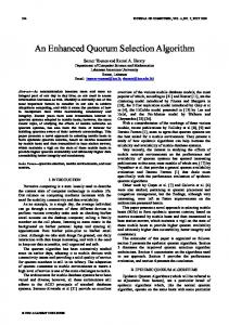
where ∆λ defines the size of the volume in the space of observables over which the stars are being counted, i.e., the resolution of the function Ψ0 . For example, one could determine the density function Ψ0 = Ψ0 (g, g − r), calculating how many stars can be found within 0.1 magnitudes of the parameter space location (g, g − r), which would mean using ∆(g, g − r) = 0.1 mag. This can be extended to any number of observables to define a “density” over multiple parameters; an example would be using additional colors, calculating the number of stars within 0.1 magnitude of (g, u − g, g − r, r − i,...). An example of a Ψ0 function can be seen in Figure 1, which shows the statistical distribution of g − r color for all stars in two sample LAMOST plates as the solid black histograms. These have been normalized so that the sum of all bins equals one, and can thus be thought of as probability functions (in this case, Ψ0 = Ψ0 (g − r)). A similar plot is seen in Figure 2 for r magnitudes in the same two plates. For the remainder of this paper, we will use examples from the simple case of the local density defined by the number of stars within 0.1 magnitudes in r, g − r and r − i, i.e. Ψ0 = Ψ0 (r, g − r, r − i). It is useful to point out that if one performs a target selection following method “A,” then the density distribution of the target stars, denoted ΨA , would be approximately the same as the statistical distribution in the input catalog, to within the Poisson errors, i.e. ΨA (λi ) ≈ Ψ0 (λi ). Typically, however, one may want to obtain a list of targets whose statistical distribution differs from the distribution in the input catalog. For instance, one may want to overselect objects in a given color/magnitude range, or pay more attention to outliers or unusual stars. One possibility, which we will call “Method B,” is to assign a selection probability that is inversely proportional to the local density in the space of observables KB , (8) Ψ0 ([λ1 ]j , [λ2 ]j , ..., [λNO ]j ) % where KB is a normalization constant to ensure that j Pj,B = 1. In Method B, the statistical distribution of the selected stars (ΨB ) over the observables (λi ) is different from that of the input Pj,B =

LEGUE Target Selection Algorithm

759

Fig. 1 Fractional distribution of g − r color for stars in two sample regions of the sky 6◦ × 6◦ in size (slightly larger than the area of a LAMOST plate); all data are selected from SDSS DR8. The left panel is for a field spanning (α, δ) = (130◦ − 136◦ , 0◦ − 6◦ ), corresponding to a field center in Galactic coordinates of (l, b) ≈ (225◦ , 28◦ ). This field contains a total of 102 199 stars between 14.0 < r < 19.5. The right panel shows a field at (α, δ) = (170◦ − 176◦ , 0◦ − 6◦ ), or (l, b) ≈ (261◦ , 59◦ ), containing a total of 44 566 stars. In both panels, the black solid line represents all stars in the field. The dashed histogram represents the stars selected by our algorithm as input to the LAMOST fiber-assignment program (∼600 per square degree), and the dash-dotted line shows the resulting distribution of spectroscopic targets in a single LAMOST plate (∼ 4000 stars assigned to fibers). Each histogram has been normalized to one, so that the bin heights represent the fraction of targets within each bin.

catalog (Ψ0 ), and in fact it is to first order uniform over all values of λi , i.e. ΨB (λi ) ≈ KB . Examples of this type of selection are seen in panels (b) of Figures 3 and 4. Note, however, that because the local density was calculated using r, g − r and r − i, the distribution does not look uniform in the color-magnitude diagrams (top and middle rows). However, the distribution in three-dimensional parameter space defined by λi = r, g − r, r − i should be roughly uniform. As a generalization, one can assign probability that is inversely proportional to some power of the local density, i.e., [Ψ0 ]−α . In this case, which we will call Method C, KC (9) [Ψ0 ([λ1 ]j , [λ2 ]j , ..., [λNO ]j )]α % where KC is a normalization constant to ensure that j Pj,C = 1. One can now see that Methods A and B represent special cases where α = 0 and α = 1, respectively. The random selection approach (α = 0) would be ideal if one simply wanted a selection that samples all of parameter space with the same frequency as the input catalog. A weighting by 1/Ψ0 (α = 1), on the other hand, produces an output catalog that samples the space of observables more evenly, and thus contains a much larger fraction of “rare” objects (i.e., those in less-populated regions of parameter space, and de-emphasizes regions of higher local density relative to the input catalog; see, e.g., panels (b) of Figs. 3 and 4). Adopting a value 0 < α < 1 would result in a selection intermediate between these two scenarios; one that increases the chances of rare objects entering the selection, but still robustly samples the high-density regions of the input distribution. The effects of using α = 1/2 are seen in panels (c) of Pj,C =

760

J. L. Carlin et al.

Fig. 2 Fractional distribution of r magnitude for stars in the same two example regions as in Fig. 1. The line styles and colors are also the same as in Fig. 1. Each histogram has been normalized so that the bin heights represent the fraction of targets within each bin; this distribution can be thought of as a probability distribution, Ψ0 (r), of finding a star in each magnitude range.

Figures 3 and 4. In the case where one would like to place a particular emphasis on rare objects, a value of α > 1 could be used, which would introduce a bias against the selection of more common objects as targets. (Also, note that if there are fewer stars in a given region of parameter space than are selected in the more densely populated regions, that region will continue to be under-dense no matter what emphasis is applied.) In any case, one may also be interested in over-selecting objects occupying a particular region of parameter space (for example, a narrow color or magnitude range, or simply selection of more blue than red stars). To achieve this, an overemphasis can be included that favors the selection of stars in a particular range of an observable by including a bias explicitly in the selection probability function. Any functional form of each of the observables, λi , can be introduced to achieve the desired effect & i fi ([λi ]j ) Pj,D = . (10) [Ψ0 ([λ1 ]j , [λ2 ]j , ..., [λNO ]j )]α Here the fi (λi ) can be any function of the observables λi . Two examples that are currently implemented for the LAMOST pilot survey are a local emphasis over a specific range of colors, and a general bias over the magnitude range to emphasize brighter stars or fainter stars. A local emphasis is achieved using a function of the form fi (λi ) = 1 + Ai e

−

(λi −xi )2 σ2 i

,

(11)

where xi is the central value of interest for the observable λi (to emphasize the center of the color or magnitude range), σi is the range of interest, and Ai is the “over-selection” factor (how strongly you wish to overemphasize these objects compared to stars outside of this range). An example is shown in panels (d) of Figures 3 and 4, where the region of interest is centered at g − r = 0.8, with a range σg−r = 0.2 and an overemphasis factor A = 10.

LEGUE Target Selection Algorithm

Fig. 3 Color-magnitude Hess diagrams for different selections of stars in the region (α, δ) = (130◦ − 136◦ , 0◦ − 6◦ ), corresponding to a field center in Galactic coordinates of (l, b) ≈ (225◦ , 28◦ ). Panel (a) shows all of the 102 199 SDSS stars between 14.0 < r < 19.5 in this field of view. Panels (b)–(e) show the results of selecting 600 stars per square degree in this field, with different selections (based on local density in three-dimensional r, g −r, r −i space, or Ψ0 (r, g −r, r −i)) represented in each panel. Panel (b) stars were selected with α = 1, and panel (c) depicts the α = 0.5 case. The α = 1 selection (i.e., weighting by the inverse of Ψ0 ) in panel (b) strongly de-emphasizes high-density regions of the CMD in favor of rare stars. M-stars at g − r ∼ 1.5 appear oversampled in this figure; this arises because they are more spread out in r − i colors than in g − r, causing them to be emphasized by the density weighting in 3-D parameter space. The overemphasis of rare objects is slightly less pronounced for α = 0.5 (panel (c)), with a significant number of stars selected from the high-density regions of the CMD. In panel (d) we illustrate the results of selection with α = 0.5 and with an over-selection of the region centered at g − r = 0.8 with width σg−r = 0.2 and overemphasis factor A = 10. This selection produces an overselection of stars centered at g − r = 0.8, while retaining some stars from the remaining parameter space. Finally, panel (e) illustrates a selection with α = 0.5 and a linear bias in color beginning at g − r = 1.1 and sloping upward toward bluer colors with slope 2.5, and also a linear magnitude emphasis beginning at r = 17.5 with slope 1.0 toward brighter magnitudes.

761

762

J. L. Carlin et al.

Fig. 4 As in Fig. 3, but for a different field located at (α, δ) = (170◦ − 176◦ , 0◦ − 6◦ ), or (l, b) ≈ (261◦ , 59◦ ). This higher-latitude field contains a total of 44 566 SDSS stars between 14.0< r 1.0. F-turnoff stars have colors of roughly 0.2 < g − r < 0.5. BHB stars (and to a lesser extent, K/M giants) occupy a region of low stellar density in colormagnitude space, while F-turnoff stars are very common. This proposed survey would also like to obtain spectra of metal-poor M subdwarfs, which are not distinguishable in the g − r band from all other M-dwarfs, but separate clearly in r − i colors, while still sampling a large number of nearby M-dwarfs that can be used to probe local kinematics. There is also interest in following up interesting discoveries with high-resolution spectroscopy, so we wish to overemphasize bright stars within reach of echelle-resolution spectrographs. Finally, there is a desire to sample all stellar populations, but preferentially observe rare objects first, in order to open up the discovery space to rare (and perhaps previously unknown) stellar types. Briefly, then, the target selection categories are as follows: – Sample a larger fraction of “rare” stars than the “less rare” cases. As shown in Section 2, this is exactly what is achieved by the use of local density weighting, Pj ∝ [Ψ0 (λi )−α ]j , in assigning selection probabilities to each star. In particular, we have shown examples of α = 1 and α = 1/2; the α = 1 case predominantly selects rarer objects (i.e., it under-emphasizes parameter spaces of high stellar density) than the α = 1/2 density weighting. – Select nearly all stars with 0.1 < (g − r) < 1.0 and r < 17 at high Galactic latitudes, and sub-sample at b < 40◦ . – Select nearly all stars with g − r < 0.0 and u − g colors that are unlike those of quasars (BHB and blue straggler candidates). – Select a significant fraction of the stars with 0.0 < (g − r) < 1.0, 17 < r < 19.5 and u − g colors that suggest they are not quasars. The bluer side of the color range should be selected with a probability about twice the redder side of the range to emphasize the F-type turnoff stars. – Select a large number of M dwarfs at all magnitudes. We note that the above discussion refers to a survey with multiple visits to each sky position, which can thus meet the requirements of nearly-complete samples of some subsets of stellar types (for example, the very blue g − r < 0 stars). However, in practice not all of the high priority targets can be placed on one observation due to constraints on fiber positioning. Thus, for a survey where only a single visit to each sky area is planned, these “requirements” should be considered to mean that one would like as many as possible of the stars in these categories. 3.2 Adopted Target Selection Parameters Through many tests, it was determined that the simplest combination of parameters striking a good balance between all these desired categories of targets is – α = 0.5, which weighs by the inverse square root of the local density. – Linear ramp bias function in g − r, beginning at g − r = 1.1 and increasing blueward with a slope of 2.5. – Linear ramp bias function in r magnitude, beginning at r = 17.5, increasing toward brighter stars with slope of 1.0. The particular values of these parameters (and particularly of α = 0.5) were determined somewhat subjectively based on visual examination of the selected targets and statistical distributions of targets

766

J. L. Carlin et al.

Fig. 5 Left panel: Color-magnitude Hess diagram of all 112 099 stars between 14 < r < 19.5 selected from SDSS DR8 at (α, δ)J2000 = (130◦ −136◦ , 0◦ −6◦ ). Center panel: Result of selecting 600 targets per square degree from the stars in the left panel. The target selection used α = 0.5 (to emphasize rare objects) with a ramp in color (to increase the fraction of blue stars selected) anchored at g − r = 1.1 and increasing blueward with slope of 2.5, and a ramp in magnitude (to weight bright stars more heavily) starting at r = 17.5 and increasing with slope of 1.0 toward the bright end. This selection represents 21.1% of the stars in the field of view. Right panel: Distribution of targets assigned to LAMOST fibers upon running the catalog from the center panel through the fiberassignment software. This panel contains a total of 3715 stars, or 3.6% of the total number within the field of view.

from separate categories (as seen in Table 1, which will be discussed in more detail below). Of course, detailed analysis could be done to optimize these target selection parameters if desired. However, in the case of a survey such as LAMOST, which will observe large numbers of stars with a variety of science goals, we simply select these parameters to produce input catalogs that are broadly consistent with the desired target distributions and sample all of parameter space to some extent. Table 1 Fraction of Stars from Each Target Category Assigned to Fibers in a Single LAMOST Plate RA (◦ )

Dec l b Total stars Assigned % Assigned Very blue Bluish, Bright Bluish, Faint Red (◦ ) (◦ ) (◦ ) (%) (%) (%) (%) (%)

133±3 3±3 225 28 173±3 3±3 261 59

102199 44566

3715 3722

3.6 8.4

22.6 27.0

6.7 15.5

2.7 6.9

2.1 5.7

3.3 Sample Target Selections In this section, we show examples of outputs from the target selection code, and follow this by selecting stars for targeting from among these using the LAMOST fiber-assignment routine. These

LEGUE Target Selection Algorithm

767

Fig. 6 As in Fig. 5, but for the higher-latitude field at (α, δ)J2000 = (170◦ − 176◦ , 0◦ − 6◦ ). This field of view contains a total of 44 566 stars, of which 48.4% were selected for the center panel. Of these, 3722 (seen in the right panel), or 8.4%, were assigned to fibers.

examples use the data from the same two fields presented earlier in this work, selected from 6 × 6◦ fields at (α, δ)J2000 = (130◦ −136◦, 0◦ −6◦ ) and (α, δ)J2000 = (170◦ −176◦ , 0◦ −6◦ ). These fields were chosen to show an example of a field at somewhat low latitude (b ∼ 30◦ ), and another at high latitude (b ∼ 60◦ ). The local density, Ψ0 , is calculated in each of these fields using r magnitudes and g − r, r − i colors. For reference, the r vs. g − r color-magnitude distribution of all 102 199 stars in the α ∼ 133◦ field of view is seen in the left panel of Figure 5, and the 44 566 stars in the lower-latitude α ∼ 173◦ field in Figure 6 (note that these are the same as panels (a) in Figs. 3 and 4). The center panels of Figures 5 and 6 show the results of running the target selection routine on the input catalogs, using α = 1/2, a linear ramp in color, beginning at g − r = 1.1 and rising blueward with slope 2.5, and a ramp in magnitude, increasing from r = 17.5 with slope 1.0 toward bright stars. These selections contain 600 stars per square degree, the required target density to be input into the fiber assignment program. In the field at α ∼ 133◦ (Fig. 5), 21.1% of the 112 099 total stars in the region were selected as candidates, and in the higher-latitude α ∼ 173◦ field (Fig. 6) this number rises to 48.4% of the total available stars. After running the catalogs selected for these two fields of view through the LAMOST fiber assignment program, ∼ 3700 stars in each of the two fields are allocated to fibers (the remaining fibers are to be used for sky and other calibration purposes). The right panels of Figures 5 and 6 show the stars assigned to fibers in these two fields. Generally, it is clear that quite a few “rare” objects (for example, at intermediate colors of 0.8 < g − r < 1.2, or bright M-star candidates at g − r ∼ 1.4) are selected by this method, but that densely-populated regions of color-magnitude space are also well-sampled. Note the fairly dramatic overemphasis of bright (r < 17), blue (g − r < 1.0) stars achieved by the weighting scheme. To assess how well the algorithm achieved the list of target selection goals outlined in Section 3.1, we select stars from the color and magnitude ranges in which specific target-selection

768

J. L. Carlin et al.

goals were focused, and explore the relative emphasis or de-emphasis achieved by our code. The degree of emphasis can be seen by comparing the fraction of stars selected within a given target category to the fraction of the total number of stars in the field. These results are given for the two example fields in Table 1. The table lists the number of stars in each of the two fields of view (“total stars”), followed by the number assigned to fibers for a single LAMOST plate (“assigned”), and the percentage of the total stars that were assigned to be observed (“% assigned,” or “assigned”/“total stars”). The following four columns represent the four categories outlined in Section 3.1: “very blue” stars with g − r < 0, “bluish, bright” stars with 0.0 < g − r < 1.0 and r < 17, “bluish, faint” stars with 0.0 < g − r < 1.0 and r > 17, and “red” stars with g − r > 1.0. In each of these columns, we provide the percentage of the total number of stars in the field that satisfy those criteria that were assigned to a fiber on the plate. This percentage can be compared to the “% assigned” column to see over- or under-emphasis; i.e., if the target selection was uniform across color-magnitude space, one would expect roughly the same fraction of stars to have been assigned in each category. Thus, for the α = 133◦ field, the fact that 22.6% of the very blue stars were assigned compared to 3.6% overall means that the “very blue” stars have been overemphasized by a factor of > 6. Examination of Table 1 shows that, at least broadly, we have achieved our goals of strongly over-selecting very blue objects, increasing the fraction of bright, blue stars that gets observed, yet still retaining a significant number of faint, bluish stars and red K- and M-star candidates (note that > 800 red stars with g − r > 1.0 were assigned in each plate – even though they have been underemphasized, they are still well-represented). 4 SOME CAVEATS ABOUT STATISTICAL TARGET SELECTION Ostensibly, one of the reasons for having a smoothly-varying, well understood selection function is to be able to infer the underlying stellar populations from a given set of spectroscopically observed stars. However, in order for this to be possible, detailed records of the entire target selection and fiber assignment process need to be kept. The first issue affecting this is the need to supply the fiber assignment routine with a catalog with higher target density than the fiber density on the sky. Because of this, not all high priority targets will be placed on fibers. Some fibers in each observation will inevitably fail to yield useful spectra, making it necessary to factor the “missed targets” into the analysis. Of course, any routine that preferentially targets certain objects will produce different target demographics if multiple visits to the same sky position are desired. An illustration of this is seen in Figure 7, which shows examples of three LAMOST plates selected in each of the two example fields used throughout this work. The upper panels show the relatively low-latitude (b ∼ 30◦ ) field, and the lower panels show the b ∼ 60◦ field. The target selection parameters were the same as those used in Sections 3.2 and 3.3, and seen in Figures 5 and 6. In each row, the five panels show r vs. g − r Hess diagrams of (a) the input sky distribution from SDSS, (b) the first plate selected, (c) the second plate selected (excluding stars from plate 1), (d) the third plate selected (excluding stars from plates 1 and 2), and (e) the sum of all three plates from (b)–(d). In the low-latitude field there are many stars available, so that the effects of the preferential targeting categories are seen in all three plates (especially the emphasis on bright, blue stars). However, the sum of all three plates (panel (e)) contains representative samples from all regions of color-magnitude space. The higher-latitude field (lower panels) is quite different. The stellar density is much lower in this field, so that in three LAMOST plates, a total of 24.4% of the stars between 14 < r < 19.5 are assigned to fibers. The first plate (panel (b)) appears very similar to the corresponding selection from the low-latitude field, with bright, blue stars overemphasized (note also that many of the very blue, g − r < 0.2 objects are gone after the first plate). By the second and third plates in this field, however, a large fraction of the bright, blue stars have already been assigned, and the selected stars start to cover more of the parameter space (specifically, there are many more faint stars – especially a lot more faint, red

LEGUE Target Selection Algorithm

769

Fig. 7 Color-magnitude Hess diagrams for stars selected from the low-latitude (b ∼ 30◦ ) field (upper panels) and high-latitude (b ∼ 60◦ ) example fields. The same target selection parameters were used as in Figures 5 and 6. In each row, the panels represent (a) all stars from SDSS in the field of view, (b) stars selected for fiber assignment on the first LAMOST plate in this field, (c) a second plate excluding the stars in the first assignment, (d) a third plate, excluding stars from the first two, and (e) the sum of the three selected plates. The high-latitude field of view contains a total of 44 566 stars, and the lower-latitude field has 102 199. Roughly 3700 stars were assigned on each of the three plates, so that in total, 24.4% of the high-latitude stars were assigned to a fiber on one of the three plates, and 10.8% of those at lower latitudes. In the low-latitude field there are many stars available, so the effects (especially the emphasis on bright, blue stars) of the preferential targeting categories are obvious in all three plates. However, the sum of all three plates (upper panel (e)) contains representative samples from all regions of color-magnitude space. The higher-latitude field (lower panels) has much lower stellar density. The first high-latitude plate (lower panel (b)) appears very similar to the corresponding selection from the low-latitude field, with bright, blue stars overemphasized (also note that many of the very blue, g − r < 0.2 objects are gone after the first plate). By the second and third plates in this field the selected stars start to cover more of the parameter space; once a large fraction of the bright, blue stars have been assigned, many more faint, red M-type stars get selected.

M-type stars). Thus if one pre-selected three plates in a high-latitude field, the demographics of the stars on each observed plate would be quite different from each other. This makes reconstruction of the underlying populations rather difficult, because a different fraction of stars from each region of parameter space will have been observed depending on the stellar populations and stellar density in each field. Of course, variations in the number of times a given piece of sky is covered will dramatically alter the distribution of objects in the final catalog.

770

J. L. Carlin et al.

Finally, we note that a routine that weights stars for selection based on the local density in parameter space will produce catalogs with different target demographics for different regions of sky. This is inevitable, because as we just showed, the stellar density on the sky actually affects the distribution of selected stars in parameter space, such that there is no way to get identical samples from regions of sky with different stellar densities. We also note that for a survey such as LAMOST, with a circular field of view, it is not possible to cover the whole sky with each part sampled only once. This will inevitably make the sampling of certain regions of sky higher than others. Thus, to determine the underlying stellar populations based on the observed spectroscopic sample, one would need to either simulate the entire selection process, or compare the number of spectra of each type observed in a given part of the sky to the number of that same type of star that was available in the photometric catalog. We note that holistic models of the Galaxy with tuneable analytic parameters are now available (e.g., the Galaxia code; Sharma et al. 2011) which could be sampled with the selection function of the survey and used to correct survey artifacts. 5 CONCLUSIONS We have presented a general target selection algorithm that can be used in any instance where large numbers of stars are to be selected from a catalog that is much larger than the desired number of targets. The program performs selections in multi-dimensional parameter space defined by any number of observables (or combinations of observables). Various functions are available to emphasize certain types of targets, and the program can be readily modified to implement an overemphasis based on any smooth function of the observables. This target selection algorithm was developed for the LEGUE portion of the LAMOST survey, and has been implemented in the LAMOST pilot survey. We have shown that careful choice of the target selection parameters can produce the desired relative numbers of various target categories, while retaining a smooth distribution across parameter space. Acknowledgements We thank the referee, Sanjib Sharma, for helpful comments on the manuscript. This work was supported by the US National Science Foundation, through grant AST-09-37523, the National Natural Science Foundation of China (Grant Nos. 10573022, 10973015 and 11061120454) and the Chinese Academy of Sciences through grant GJHZ 200812. S. L. is supported by the US National Science Foundation grant AST-09-08419. References Aihara, H., Allende Prieto, C., An, D., et al. 2011, ApJS, 193, 29 Allende Prieto, C., Beers, T. C., Wilhelm, R., et al. 2006, ApJ, 636, 804 Barden, S. C., Bland-Hawthorn, J., Churilov, V., et al. 2008, in Society of Photo-Optical Instrumentation Engineers (SPIE) Conference Series, 7014 Belokurov, V., Zucker, D. B., Evans, N. W., et al. 2006, ApJ, 642, L137 Carollo, D., Beers, T. C., Lee, Y. S., et al. 2007, Nature, 450, 1020 Chen, Y. Q., Zhao, G., Carrell, K., & Zhao, J. K. 2011, AJ, 142, 184 Chen, L., Hou, J., Yu, J., et al. 2012, RAA (Research in Astronomy and Astrophysics), 12, 805 Cheng, J. Y., Rockosi, C. M., Morrison, H. L., et al. 2012, ApJ, 746, 149 Deng, L., Newberg, H. J., Liu, C., et al. 2012, RAA (Research in Astronomy and Astrophysics), 12, 735 Dierickx, M., Klement, R., Rix, H.-W., & Liu, C. 2010, ApJ, 725, L186 Freeman, K. C. 2010, in Galaxies and their Masks, eds. D. L. Block, K. C. Freeman, & I. Puerari, 319 Freeman, K., & Bland-Hawthorn, J. 2008, in Astronomical Society of the Pacific Conference Series, 399, Panoramic Views of Galaxy Formation and Evolution, eds. T. Kodama, T. Yamada, & K. Aoki, 439 Grillmair, C. J., & Dionatos, O. 2006, ApJ, 643, L17 Klement, R., Rix, H.-W., Flynn, C., et al. 2009, ApJ, 698, 865

LEGUE Target Selection Algorithm Lee, Y. S., Beers, T. C., An, D., et al. 2011, ApJ, 738, 187 Newberg, H. J., Yanny, B., Rockosi, C., et al. 2002, ApJ, 569, 245 Newberg, H. J., Yanny, B., Cole, N., et al. 2007, ApJ, 668, 221 Schlaufman, K. C., Rockosi, C. M., Allende Prieto, C., et al. 2009, ApJ, 703, 2177 Sharma, S., Bland-Hawthorn, J., Johnston, K. V., & Binney, J. 2011, ApJ, 730, 3 Smith, M. C., Evans, N. W., Belokurov, V., et al. 2009, MNRAS, 399, 1223 Smith, M. C., Whiteoak, S. H., & Evans, N. W. 2012, ApJ, 746, 181 Steinmetz, M., Zwitter, T., Siebert, A., et al. 2006, AJ, 132, 1645 Xue, X. X., Rix, H. W., Zhao, G., et al. 2008, ApJ, 684, 1143 Xue, X.-X., Rix, H.-W., Yanny, B., et al. 2011, ApJ, 738, 79 Yang, F., Carlin, J. L., Liu, C., et al. 2012, RAA (Research in Astronomy and Astrophysics), 12, 781 Yanny, B., Newberg, H. J., Grebel, E. K., et al. 2003, ApJ, 588, 824 Yanny, B., Rockosi, C., Newberg, H. J., et al. 2009a, AJ, 137, 4377 Yanny, B., Newberg, H. J., Johnson, J. A., et al. 2009b, ApJ, 700, 1282 Zhang, Y., Carlin, J., Liu, C., et al. 2012, RAA (Research in Astronomy and Astrophysics), 12, 792 Zhao, G., Zhao, Y., Chu, Y., et al. 2012, RAA (Research in Astronomy and Astrophysics), 12, 723

771