An Algorithm for Stereotype Deduction in UML-Based Formalism and its Application in Geographic Information Systems François Pinet, Ahmed Lbath Laboratory of Information System Engineering, INSA Lyon, 69621 Villeurbanne Cedex, France, and CIRIL SA, 69100 Villeurbanne, France.
[email protected],
[email protected] Abstract Stereotypes provide a mechanism for extending the vocabulary of the UML. Present UML-based formalisms for Geographic Information System use the concept of visual stereotypes in order to represent geographic types. This paper extends the expressiveness of stereotypes currently defined for geographic types and describes an algorithm for the computation of visual stereotypes resulting from aggregation operations.
as networks, maps, tessellation, etc. This is the reason why disjunctive and conjunctive operations were introduced in object-oriented formalisms for GIS [4][5][7][8][9]. Using these operations, stereotypes associated to a simple geographic type can be visually combined in order to provide a more complex geographic type. The visual representation of the conjunctive and disjunctive operations considered in this paper is described in figure 2 (see [9]). The result of these operations is a combined stereotype.
1. Introduction UML Notation:
Numerous conceptual modelling methods for Geographic Information Systems (GIS) have been proposed in the recent years. Their goal is to provide a design process and a specific formalism suitable for GIS. Some of these modelling methods are even supported by CASE Tool prototypes or by marketed CASE Tools [1][4][6][10][11]. These methods enable GIS designers to easily and clearly specify aspects related to geographic information. For that, these methods use visual representations that are easily understandable by GIS designers. Most of proposed formalisms are presented as extensions of the UML class diagram [2]. These object-oriented methods for GIS usually integrate the concept of geographic class i.e. a class having access to a geographic attribute. A geographic class inherits diverse operations (intersect, setBounds, etc) depending on the type of its geographic attribute [6]. In order to provide an explicit representation of these types, almost all objectoriented methods for GIS associate each geographic type to a visual stereotype 1. For example, in the small class diagram presented in figure 1, the class Frontier has a geographic attribute of type polygon and the class River has a geographic attribute of type polyline. Unfortunately, such geographic types are not efficient to model geographic objects with complex structures, such 1
The first method that introduced a visual representation for geographic types is the entity-relationship method MODUL-R [1]. Afterwards this type of visual representation has been reused in the object-oriented methods GeoFrame [5], GeoOOA [6], GeoUML [4], OMEGA [7][8][10][12], OMT-G [3] and MADS [11].
0..*
Country
aggregation inheritance
Capital_Town
1..1
1..1
0..*
1..1
xor
Frontier Capital_Town_Representation2 River Capital_Town_Representation1
Figure 1. Class Diagram using Stereotypes
Disjunction Operation: the value of the geographic attribute is either a point or a polygon but not both
Conjunction Operation: the value of the geographic attribute is composed of a point and a polygon
Figure 2. Conjunction and Disjunction Operations The present methods for GIS modelling define a finite number of stereotypes. Indeed, they often don’t allow the combination of more than two simple stereotypes. For example, the combination of one point and one polygon is allowed but not the combination of one point and one polygon and one polyline. Thus, this constraint makes the specification of several geographic objects difficult. In this paper, the definition of stereotypes resulting from an unlimited number of combinations will be studied. Thus, it will become possible to express very complex geographic types (for example, geographic types that
result from aggregation). This paper will give a precise definition of the stereotypes set. In order to know the exact semantics of stereotypes, a function that associates a value domain to each stereotype will be presented. Also, this paper will use the concept of multiplicity related to stereotypes (introduced in [4]). On the other hand, GIS designers have to define aggregation relationships between geographic classes [3][4][5]. The aggregation is one of the most important operations in GIS modelling because of its direct repercussion on the geographic type of classes. In the class diagram of figure 1, an aggregation relationship is defined between a whole and its parts. In this example, a country (the whole) is composed of a frontier (a polygon), zero, one or many rivers (polylines), and a capital town (represented by either a point or a polygon but not both); according to the UML notation, a xor relation can link two aggregation relationships [2]. The type of the geographic attribute associated to the class Country (the whole class) is represented by a stereotype. This stereotype uses the new formalism presented in this paper, and corresponds to the aggregation of the types related to part geographic attributes. The multiplicity [0..*] is also introduced in the polyline stereotype of the whole; it means that the whole contains from zero to + ∞ polylines. At the conceptual level, it is very interesting for GIS designers to exactly know the geographic type resulting from an aggregation and the corresponding stereotypes. Indeed, this functionality can help designers to avoid conceptual errors in class diagrams. This paper presents an algorithm computing stereotypes associated to the whole class of an aggregation. This algorithm automatically simplifies conjunctions of stereotypes; for example, the conjunction of two polygon stereotypes produce a single polygon stereotype having a multiplicity equal to two. A specific process improving the visual representation of stereotypes resulting from the algorithm will be also described. The work presented in this paper is part of the industrial AIGLE project. AIGLE is a CASE-Tool that supports the OMEGA method [7][8][10][12]. AIGLE is marketed by the French Company CIRIL SA and OMEGA is an object-oriented method for GIS. The final goal is to integrate the presented work into OMEGA and AIGLE in order to generate automatically geographic data structures resulting from aggregation operations.
2. Visual representation of geoTypes 2.1 Notation The presented formalism uses two types of unordered collections: the set and the bag. The set doesn’t contain duplicate elements; any element can be represented only
once. A set is denoted by {element1,…,elementn}. Let S be a set, 2S is the set of all subsets of S. The size of a set is its number of elements denoted by |S|. A bag is similar to a set, but it can contain duplicate elements; that is, the same element can occur in a bag more than once. A bag is denoted by Bag{element1,…,elementn}. The empty bag is Bag{}. The combination of bags is allowed by using the union operator. For example, Bag{a,b} ∪ Bag{b,c} ∪ Bag{} = Bag{a,b,b,c} The cross-product (denoted by ×) provides the capability for combining sets of bags. The cross-product of two sets of bags S1 and S2 is S1 × S2 = { Bagi ∪ Bag ′j | Bagi ∈ S1 and Bag ′j ∈ S2 } For example, {Bag{a,b},Bag{c}}×{Bag{c}}={Bag{a,b,c}, Bag{c,c}} The cross-product is associative. Also, because the bag is an unordered collection, the cross-product on sets of bags is commutative. S n is the cross-product of S with itself n times; if applied to cross-product on a set of bags, 0 1 2 3 S = {Bag{}} ; S = S ; S = S × S ; S = S × S × S ; ...
2.2 Geographic domains and simple geoTypes In class diagrams of object-oriented methods for GIS, each class has one (and only one) geographic attribute and a stereotype that represents the geographic type of this attribute. The value of a geographic attribute is an unordered collection (more precisely a bag) of geographic objects. This subsection describes simple geographic types considered in this paper. In the following, geographic types will be called geoTypes and geographic attributes will be named geoAttributes. The simple geoTypes considered in this paper are: point[min..max], polyline[min..max], polygon[min..max], [min..max] circle . Their domain of values is the set composed of bags that contain respectively from min to max points, polylines, polygons, or circles. Let Dom(t) be the domain of values related to a geoType t. Each geoAttribute having a geoType t must match with one and only one value in Dom(t). For example, Dom(circle[1..1]) is the infinite set of bags that contain one circle and Dom(circle[2..2]) is the infinite set of bags that contain two circles. Thus, Dom(circle[0..2]) = {Bag{}} ∪ Dom(circle[1..1]) ∪ Dom(circle [2..2]) = {Bag{}, Bag{circle1}, … , Bag{circlei}, … , Bag{circle1, circle1}, … , Bag{circlei, circlej}, …} Consequently, the value of a geoAttribute having the type circle[0..2] must be a bag included in the above set. For each t ∈ {point, polyline, polygon, circle}, Dom(t[i..m]) = Dom(t[i..i]) ∪ …∪ Dom(t[k..k]) ∪ …∪ with i≤k≤m Dom(t[m..m]) Moreover, the following notation equivalencies are considered: t [i] = t [i..i] ; t [i..*] = t [i..+∞] ; t [ ] = t [1..1]
[] [1..1] point = point For example, ; [2] [2..2] [0..*] point = point ; circle = circle[0.. +∞]
provide the same result. The figure 6 exemplifies an evaluation of DomSType .
2.3 Definition of simple and combined stereotypes .. 1 2 3 4 5 6 7 8 9 0 *
In most object-oriented formalisms for GIS, each simple geoType is visually represented in class diagrams by a simple stereotype. Figure 3 presents the correspondence between simple geoTypes and simple stereotypes. A more generic syntax is needed in order to define all correct stereotypes (combined or not). Thus, the definition 1 presents rules for the construction of all correct stereotypes on a set of visual constants. Notice that the notation equivalencies presented in the subsection 2.2 are also applied on multiplicity of stereotypes; for example, the point stereotype of figure 5.a has a multiplicity equal to [1..1], and the circle stereotype has a multiplicity equal to [2..2]. Stereotypes geoTypes
x..y
x..y
x..y
Figure 4. Set A of Visual Constants
2
2
0..* 0..*..
b.
a.
Figure 5. Elements of A*
x..y
1..1
1..1
0..*
1..1
point[x..y] polyline[x..y] polygon[x..y] circle[x..y] d3 (variable x)
Figure 3. Description of geoTypes
d3 (variable y) 1..1 0..*
DEFINITION 1. Let A be the set of visual constants presented in figure 4. Let A* be the set of all visual combinations of elements included in A. Dotted (open) rectangles represent (open) rectangles of all sizes. Let Geograph be the infinite set of all syntactically correct stereotypes. Geograph is a subset of A* and it is constructed only by the rules of table 1. Examples 5.a and 5.b are elements of A*, but only the example 5.a is an element of Geograph . Another step is to define the function DomSType that associates a value domain to an element of Geograph . DEFINITION 2. The definition of DomSType is given in table 2. In fact, DomSType provides the exact semantics of stereotypes. Let G1, G2 ∈ Geograph ; G1 and G2 have the same semantics iff DomSType(G1) = DomSType(G2). The function DomSType decomposes the value domain of a stereotype into cross-products and unions of simple geoType domains. The cross-product corresponds to a conjunction between value domains and the union is a disjunction between value domains. Remember that because a bag is an unordered collection, the crossproduct on sets of bags is associative and commutative. Thus, all evaluations of DomSType with a specific input
1..1 1..1
d3 (x), d1 (x) d3 ( y) 1..1
d6 (x)
0..*
d5 (x)
d2 (x) 1..1
d4 (x)
d2 ( y) 1..1
d6 (x)
Dom(polygon [1..1]) ×Dom(polyline [0..*])×(Dom(point [1..1])∪Dom(polygon [1..1]))
Figure 6. Evaluation of Dom SType In summary, Geograph is the set of all correct stereotypes (combined or not), and DomSType is a function that associates a value domain to an element of Geograph.
3. Aggregation 3.1 Definition In class diagrams, most classes collaborate with others in a number of different ways. This collaboration can be formulated by associations (also called relationships). Aggregation is a special form of association between instances, where one of them (the whole) is assembled
x ∈ Geograph if x ∈ Disjgraph ∪ Conjgraph
x
x y
∈ Disjgraph if x, y ∈ Disjgraph ∪ Conjgraph
x
x
∈ Disjgraph if x ∈ Simplegraph
i .. j , i , ∅ ∈ Mult if i ∈ N ∧ ( j ∈ N ∪ {*})
x
y
∈ Conjgraph if x ∈ Conjgraph ∧ y ∈ Disjgraph
y
∈ Conjgraph if x, y ∈ Disjgraph
x
x
x ,
,
,
∈ Simplegraph if x ∈ Mult
Table 1. Rules defining Geograph
d1. DomSType (
x
x d4. DomSType ( ) = Dom(point[x]) if x ∈ Mult
)= DomSType(x)
x d2. DomSType ( y ) = (DomSType(x) ∪ DomSType( y)) if x ∉ Mult
d5. DomSType ( d6. DomSType (
d3. DomSType ( x
y
) = (DomSType(x) × DomSType( y)) d7. DomSType (
x
) = Dom(polyline[x]) if x ∈ Mult
x
) = Dom(polygon[x]) if x ∈ Mult
x
) = Dom(circle[x]) if x ∈ Mult
Table 2. Definition of Dom SType from others (the parts). In this subsection, a function will be defined in order to determine the domain related the geoAttribute of the whole class from domains associated to the geoAttributes of the part classes. Formal structure. The first step is to describe a formal structure for aggregation associations and xor relations existing between them. DEFINITION 3. Let P(C′ ) = {R1(C1, min1, max1), … , Rn(Cn, minn, maxn)}. P(C′ ) is the set of relationships aggregating a class C′. For each relationships Ri , the part class is Ci and mini, maxi are the multiplicity implied in Ri . Let X(C′ ) = { {Ri , Rj},…,{Ru , Rv} }. X(C′ ) is the set of all binary relations xor between distinct elements of P(C′ ). Because binary xor relations are symmetric and irreflexive, elements of X(C′ ) are sets having a size equal to 2. In the example of figure 1, P(Country) = { R1(Capital_Town_Representation1, 1, 1), R2(Capital_Town_Representation2, 1, 1), R3(Frontier, 1, 1), R4 (River, 0, +∞) } X(Country) = { {R1, R2} } DEFINITION 4. Let SType be a function that takes as parameter an element Ri of P(C′ ), and returns the stereotype of the class Ci associated to Ri ; this function returns an element of Geograph .
DEFINITION 5. Let Domclass = SType • DomSType ; the composition of SType followed by DomSType . If we consider R4 ∈ P(Country), Domclass(R4) = DomSType(SType(R4)) = Dom(polyline[ ]) Multiplicity effect 2. The second step is to study the effect of the multiplicity on a domain of a geoType. This is given by the function Dommult . DEFINITION 6. Let R(C, min, max) be an element of P(C′ ), Dommult(R) = Domclass(R)min ∪ … ∪ Domclass(R)k ∪ … ∪ Domclass(R)max with min≤k≤max If we consider R4 ∈ P(Country) , Dommult(R4) = Dom(polyline[ ])0 ∪ Dom(polyline[ ])1 ∪ Dom(polyline[ ])2 ∪ Dom(polyline[ ])3 ∪ … = Dom(polyline[0..*]) Intuitively, the application of the multiplicity [0..*] on Dom(polyline[ ]) (e.g. part value domain) returns Dom(polyline[0..*]) (e.g. the whole value domain). Link between the whole and its parts. The last step is to precisely define the link between the value domain of the whole and the value domain of its parts. 2
In some cases, the presented stereotypes syntax can only offer an acceptable approximation of the multiplicity effect. A more complex syntax is required to obtain the exact semantics (see [13] for details).
DEFINITION 7. Let Q¬xor(C′ ) and Qxor(C′ ) be two sets of sets. Each element of Q¬xor(C′ ) is composed of an association not implied in a xor relation. Q¬xor(C′ ) = { {Ri} | Ri ∈ P(C′ ) and ∀S ∈ X(C′ ), Ri ∉ S } Each element of Qxor(C′ ) is composed of associations implied in a xor relation. Qxor(C′ ) ⊆ 2P(C′ ). Let S ∈ 2P(C′ ), S ∈ Qxor(C′ ) iff (∀Ri , Rj ∈ S such as Ri ≠ Rj , {Ri , Rj} ∈ X(C′ )) and (∀Ri ∈ P(C′ ) such as Ri ∉ S, ∃Rj ∈ S such as {Ri , Rj} ∉ X(C′ )) and |S| ≥ 2 Let Q(C′ ) = Q¬xor(C′ ) ∪ Qxor(C′ ) . Thus, Qxor(C′ ) assembles binary xor relations in order to compose sets of n-arity xor relations. For example, if X(C′ ) = { {Ra, Rb}, {Ra, Rc}, {Rb, Rc} } then Qxor(C′ ) = { {Ra, Rb, Rc} } In the previous example, Q¬xor(Country)={{R3},{R4}};Qxor(Country) = {{R1, R2}} Q(Country) = {{R3}, {R4}, {R1, R2}} Finally, the value domain of the geoAttribut associated to a whole class can be defined from its parts by the function Domwhole . This function is defined below and takes as parameter Q(C′ ). DEFINITION 8. Let Q(C′ ) = { {R11, … ,R1m}, … , {Rnp, … ,Rnq} }, Domwhole(Q(C′ )) = (Dommult(R11) ∪…∪ Dommult(R1m)) × … × (Dommult(Rnp) ∪…∪ Dommult(Rnq)) More intuitively, Q(C′ ) can be viewed as a conjunctive normal form of associations. Indeed, conjunction operations link the elements of Q(C′ ) and disjunction operations link elements of each set that is included in Q(C′ ). In the previous example, the geoAttribute value of a Country instance is composed of a polygon issued from R3 and polylines issued from R4 and (a point issued from R1 (exclusive) or a polygon issued from R2). Also, the function Domwhole applies the multiplicity on the value domain associated to the geoAttribut of each part class by using the function Dommult . For example, Domwhole(Q(Country)) = Dommult(R3) × Dommult(R4) × (Dommult(R1) ∪ Dommult(R2)) Thus, Domwhole(Q(Country)) = Dom(polygon[ ]) × Dom(polyline[0..*]) × (Dom(point[ ]) ∪ Dom(polygon[ ])) To summarise this subsection, P(C′ ) and X(C′ ) are the formal structures of an aggregation. C′ is the whole class. Domwhole is a function that determines the value domain of the geoAttribute associated to C′.
Domwhole uses the function Dommult and the set Q(C′ ) constructed from P(C′ ) and X(C′ ).
3.2 Automatic generation of stereotypes The purpose of this subsection is to define an algorithm for the automatic generation of stereotypes associated to C′. For that, the theoretic foundation presented in the previous section will be used. It is not possible to generate stereotypes associated to C′ in computing directly cross-products and unions of infinite value domains. This means that DomSType and Domwhole are not computable functions. Thus, each value domain (which will be called concrete domain) will be replaced by an abstract domain in all the definitions of the previous subsection. These abstract domains are finite representations of concrete domains. The operation × will be also replaced by an abstract operator on abstract domains. The final goals are to compute the abstract domain of C′ and to convert it into stereotypes. DEFINITION 9. Let D be a concrete domain i.e. a domain related to a stereotype of Geograph . Because each concrete domain can be decomposed into cross-products and unions of simple geoTypes, D = D1 ∪ … ∪ Dn with Di = Dom(point[p..q]) × Dom(polyline [r..s]) × Dom(polygon[u..v]) × Dom(circle[x..y]) This type of representations is called decomposed representation of a concrete domain. Each concrete domain has a smallest decomposed representation; the decomposed representation that has the fewest union operators. For example the smallest decomposed representation of Domwhole(Q(Country)) is (Dom(point[0]) × Dom(polyline [0..*]) × Dom(polygon[2]) × Dom(circle[0])) ∪ (Dom(point[ ]) × Dom(polyline [0..*]) × Dom(polygon[ ]) × Dom(circle[0])) DEFINTION 10. The general form of an abstract domain is a set of sets, {S1 , … , Sn} Each Si is a set of simple geoType names. The general form of Si is {point[p..q] , polyline [r..s] , polygon[u..v] , circle[x..y]} Let AbstDom be the abstraction function of concrete domains. This function takes a concrete domain D as parameter and returns its abstract domain.
AbstSType (
x
)= AbstSType(x)
AbstSType ( yx ) = (AbstSType(x) ∪ AbstSType( y)) if x ∉ Mult ) = (AbstSType(x) ⊗ AbstSType( y)) AbstSType ( x y
{ {point[0],polyline [0..*],polygon[2] ,circle[0]}, {point[ ] ,polyline [0..*],polygon[ ],circle[0]} }
x
AbstSType ( ) ={{point[x],polyline[0],polygon[0],circle[0]}} if x ∈ Mult AbstSType (
x x
AbstSType ( AbstSType (
x
0
0..*
2
0
) ={{point ,poyline ,polygon ,circle }} if x ∈ Mult [0]
[x]
[0]
[0]
0..*
) ={{point[0],polyline[0],polygon[x],circle[0]}} if x ∈ Mult ) ={{point[0],polyline[0],polygon[0],circle[x]}} if x ∈ Mult
0
Figure 7. A Visual Representation of an Abstract Domain
Table 3. Definition of AbstSType If the smallest decomposed representation of D is (Dom(t11[d..e]) × … × Dom(t1m[f..g])) ∪ … ∪ (Dom(tnp[h..i]) × … × Dom(tnq[j..k])) then AbstDom(D) = {{t11[d..e],…, t1m[f..g]},…,{tnp[h..i],…, tnq[j..k]}}
DEFINITION 13. (abstraction of definition 2) The abstraction of DomSType is called AbstSType ; its definition is given in table 3. Two stereotypes called G1 and G2 have the same semantics iff AbstSType(G1) = AbstSType(G2).
In fact, the name of a simple geoType is used as a finite representation of its value domain. Intuitively, AbstDom returns the smallest decomposed representation of a concrete domain in which the domains of simple geoTypes are replaced by names of geoTypes. For example, AbstDom(Domwhole(Q(Country))) = { {point[0],polyline [0..*],polygon[2],circle[0]} , {point[ ],polyline [0..*],polygon[ ],circle[0]} } Abstract domains provide an excellent form for the application of a cross-product abstraction. The abstract operation of × is denoted by ⊗. This abstract operation is used to compute a cross-product of abstract domains. The operation ⊗ uses an operation denoted by ⊕.
AbstSType returns the abstract domain of a stereotype. The definition of AbstSType is similar to the one of DomSType except that the operation × is replaced by ⊗ and concrete domains of simple geoTypes are replaced by their abstract domains.
DEFINTION 11. Let ⊕ be an operation on two sets included in abstract domains. {t1[i..j] , … , t4[m..n]} ⊕ {t1[p ..q] , … , t4[u..v]} = {t1[i+p..j+q] , … , t4[m+u..n+v]} For example, {point[ ],polyline [0..*],polygon[0],circle[5..8]} ⊕ {point[ ],polyline [1..10],polygon[2],circle[1..7]} = {point[2],polyline [1..*],polygon[2],circle[6..15]} DEFINITION 12. Let ⊗ be an operation on two abstract domains A and A′ . A ⊗ A′ = {Si ⊕ S′j | Si ∈ A and S′j ∈ A′ }
DEFINITION 14. (abstraction of definition 5) Let Abstclass = SType • AbstSType ; the composition of SType followed by AbstSType . An abstraction of the multiplicity effect (given by Dommult) must also be defined in order to compute the whole abstract domain. DEFINITION 15. (abstraction of definition 6 ) Let R(C, min, max) be an element of P(C′ ). Abstmult (R) returns Abstclass(R) in which each multiplicity [i..j] is replaced by [i∗min..j∗max]. For R4 ∈ P(Country), Abstclass(R4) = { {point[0],polyline [ ],polygon[0],circle[0]} } and Abstmult(R4) = { {point[0],polyline [0..*],polygon[0],circle[0]} } The abstract domain of the geoAttribut associated to a whole class is computed by the abstraction of Domwhole . DEFINITION 16. (abstraction of definition 8) Let Q(C′ ) = { {R11, … ,R1m}, … , {Rnp, … ,Rnq} }, Abstwhole(Q(C′ )) = (Abstmult(R11) ∪…∪ Abstmult(R1m)) ⊗ … ⊗ (Abstmult(Rnp) ∪…∪ Abstmult(Rnq))
T11
F1
T21
T31
Conjunction group 1
T41
F2
F3
F4
... T1n
T2n
Factor T1´1
T3n
Conjunction group n
T4n
Factorised representation Fact(G ′ )
T2´1
T3´1
T4´1
Factorised part
... T1´n
Visual representation G ′ of an abstract domain Tij = [Tij.min ..Tij.max]; Fi = [Fi.min .. Fi.max]; Ti´j = [Ti´j.min .. Ti´j.max]
T2´n
T3´n T4´ n
Translation from G ′ to Fact(G ′ ): /*compute the multiplicity F1, F2, F3, F4 of the factor: */ for 1≤i≤4 do { if ∃Tij such as Tij.min = MIN(Ti1.min,…,Tin.min) and Tij.max = MIN(Ti1.max,…, Tin.max) then Fi = Tij else Fi = [0..0]; } if each Fi is equal to [0..0] then the factorisation is unavailing; /*compute the multiplicity Ti´j of the factorised part: */ for 1≤i≤4 do for 1≤j≤n { if Fi.max = +∞ then Ti´j = [Tij.min - Fi.min .. Tij.min - Fi.min] else Ti´j = [Tij.min - Fi.min .. Tij.max - Fi.max]; if Ti´j.min > Ti´j.max then the factorisation is unavailing; }
Figure 8. Simplification of Stereotypes (step 1): definition
Abstwhole is applied on this aggregation 2..*
2..*
1..*
1..*
2..*
1..*
1..* 4..4
5..5
0..0
1..*
4..4
1..*
4..4
0..0
5..5
1..1
1..1
Stereotype G1 ′ of the aggregation
0..* 0..*
;
;
0..*
; 1..*
0..0
1..1
1..1
Fact( G1 ′ ) 2..*
1..15
Aggregation of stereotypes issued from six different classes:
Factorisation of all conjunction groups
0..0
0..0
1..1
0..0
1..1
0..0
0..0
1..1
0..0
1..1
1..*
0..5
;
;
4..4
Factorised conjunction group1
0..0
Factorisation of the first and the second conjunction groups
Factorised conjunction group2
0..0
1..1
1..1
Factorisation of the third and the fourth conjunction groups
Stereotype G2′ The end of the first factorisation process has been reached. G2′ is the result after the deletion of simple stereotypes having the multiplicity [0..0]. The semantics of this new stereotype G2′ are exactly equivalent to the semantics of G1′ because:
AbstSType(G1′) = AbstSType(G2′)
Figure 9. Simplification of Stereotypes (step 1): exemple Considering a simple example, Abstwhole(Q(Country)) = { {point[0],polyline [0],polygon[ ],circle[0]} } ⊗ { {point[0],polyline [0..*],polygon[0],circle[0]} } ⊗ ( { {point[ ],polyline [0],polygon[0],circle[0]} } ∪ { {point[0],polyline [0],polygon[ ],circle[0]} } ) = { {point[0],polyline [0..*],polygon[2],circle[0]}, {point[ ],polyline [0..*],polygon[ ],circle[0]} } As presented in figure 7, the transformation of the resulting abstract domain into a stereotype is trivial. The algorithm generating stereotypes from an aggregation is: generatingST{ /*input: P(C′ ), X(C′ );output: a stereotype*/ 1.compute Q(C′ ) from P(C′ ) and X(C′ ); 2. compute Abstwhole(Q(C′ )); 3. transform the result obtained in 2 into a stereotype; }
3.3 Visual simplification of stereotypes Step 1: factorisation of simple stereotypes. The general form of the stereotype that results from the previous algorithm is a disjunction of conjunctions (as presented in figure 7). This form can be easily simplified by using the function Fact (figure 8). The goal of this function is to factorise elements of disjunction in order to generate simple stereotypes having a multiplicity equal to [0..0]. These simple stereotypes can be removed. If each multiplicity of a conjunction group in a factorised part is equal to [0..0] then the conjunction group is replaced by a simple stereotype having a multiplicity equal to [0..0]. In this case, the choice of the type (point, polyline, etc) associated to this simple
stereotype is not important. The simplification of the stereotype presented in figure 7 gives the stereotype of the class Country presented in figure 1. If the disjunction to simplify contains more than two conjunction groups (n>2 in figure 8), the function Fact can be applied on each set of conjunction groups. For example, if the number of conjunction groups is equal to four then it is possible to factorise the four conjunction groups but also only the first one and the second one, or only the second one and the third one, etc. Then, Fact can be applied recursively on the factorised part of results. When all possible factorisations have been computed, the end of the factorisation process has been reached. At this moment, all simple stereotypes having a multiplicity equal to [0..0] can be removed. At end of this first factorisation process, several stereotypes have been generated. Figure 9 presents a possible factorisation of a complex aggregation. Step 2: factorisation of complex stereotypes. At the end of the previous process, factorised conjunction groups can be simplified. Indeed, the last part of these groups is a combined stereotype (called CS) that can be repeated in several factorised conjunction groups. For example, in the stereotype G2′ (figure 9), all factorised conjunction groups have a common combined stereotype (a disjunction between a line and a polygon). Thus, at the end of the previous factorisation process (step 1), the simplification described in figure 10 can be applied on each factorised conjunction group of each generated stereotype. Figure 10 also presents the simplification related to factorised conjunction groups of G2′. x1
CS ...
xn
CS
x1, …,xn are conjunctions
CS x1 ... xn
Example
Figure 10. Simplification Process (step 2) All possible factorisations are produced by the first simplification process. Thus, the designer has to choose one specific stereotype. If the number of generated representations is too high, only stereotypes having the fewest simple stereotypes (i.e. the best factorisation) could be proposed to the designer. It is also possible to automatically stop the program after m factorisations in order to limit the number of generated stereotypes.
4. Conclusion The first contribution of this paper is to provide a function that computes an abstract form of the semantics associated to a stereotype. Thus, it becomes possible to know if two stereotypes have exactly the same semantic.
The second contribution of this paper is to provide an algorithm for the computation of stereotypes resulting from aggregation. The problem was to find stereotypes having few redundant subparts. The proposed approach consists in factorising visual representations of abstract domains in order to find the best stereotypes i.e. the most “compacted” ones. Several experiments have yielded very good results. But heuristics are needed for large aggregations, so that most of the time the algorithm only computes factorisations leading to the most compacted stereotypes. The integration of the algorithm into AIGLE is being investigated. This paper focuses on geographic types by reason of the AIGLE project. But the presented method can be easily applied in other fields simply by replacing types or by changing visual notations.
References [1] Y. Bedard, C. Caron, Z. Maamar, B. Moulin, D. Valliere, "Adapting Data Models for the Design of Spatio-Temporal Databases", Computer, Environment and Urban Systems Int. Journal, vol.20(1), 1996, pp.19-41. [2] G. Booch, J. Rumbaugh, I. Jacobson, The Unified Modeling Language User Guide, Addison-Wesley, 1999. [3] K. Borges, A. Laender, D. Clodoveu, "Spatial Data Integrity Constraints in Object Oriented Geographic Data Modeling", in Proc. of the Int. Symposium on GIS, ACM Press, USA, 1999, pp.1-6. [4] J. Brodeur, Y. Bedard, M. Proulx, "Modelling Geospatial Databases using UML-based Repositories Aligned with International Standards in Geomatics", in Proc. of the Int. Symposium on GIS, ACM Press, USA, 2000, pp.39-46. [5] L.F. Jugurta, L. Cirano, "Specifying Analysis Patterns for Geographic Databases on the Basis of a Conceptual Framework", in Proc. of the Int. Symposium on GIS, ACM Press, USA, 1999, pp.7-13. [6] G. Kösters, B. Pagel, H. Six, "GIS-Application Development with GeoOOA", Int. Journal of Geographical Information Science vol.11(4), 1997, pp.307-335. [7] R. Laurini, Information Systems for Urban Planning, Taylor & Francis Press, 2001. [8] A. Lbath, AIGLE: a Visual Environment for Design and Automatic Generation of Geographic Applications, Phd Thesis, INSA Lyon, France, 1997. [9] A. Lbath, F. Pinet, "Towards Conceptual Modelling of TeleGeoProcessing Applications", in Proc. of the Int. Symposium on TeleGeoProcessing, France, 2000, pp.25-39. [10] A. Lbath, F. Pinet, "The Development and Customization of GIS-Based Applications and Web-Based GIS Applications with the CASE Tool AIGLE" (industrial track), in Proc. of the Int. Symposium on GIS, ACM Press, USA, 2000, pp.194-196. [11] C. Parent, S. Spaccapietra, E. Zimanyia, "Spatio-Temporal Conceptual Models: Data Structures + Space + Time", in Proc. of the Int. Symposium on GIS, ACM Press, USA, 1999, pp.26-33. [12] F. Pinet, A. Lbath, "A Visual Modelling Language for Distributed Geographic Information Systems", in Proc. of Int. Symposium on Visual Languages, IEEE, USA, 2000, pp.75-76. [13] F. Pinet, A. Lbath, "Stereotypes in UML-Based Formalism", Technical Report, LISI INSA Lyon, France, 2001.


![PAYROLL DEDUCTION I hereby authorize payroll deduction for [PDF]](https://m.moam.info/img/260x300/payroll-deduction-i-hereby-authorize-payroll-deduc_64865a59098a9eb05f8b4592.jpg)