An Algorithm for the Graph Crossing Number Problem [Extended Abstract] ∗
Julia Chuzhoy
Toyota Technological Institute, Chicago, IL 60637
[email protected] ABSTRACT We study the Minimum Crossing Number problem: given an n-vertex graph G, the goal is to find a drawing of G in the plane with minimum number of edge crossings. This is one of the central problems in topological graph theory, that has been studied extensively over the past three decades. The first non-trivial efficient algorithm`for the ´problem, due to Leighton and Rao, achieved an O n log4 n -approximation for bounded degree graphs. This algorithm has since been improved by poly-logarithmic factors,“with the best current ” approximation ratio standing on O n · poly(d) · log3/2 n for graphs with maximum degree d. In contrast, only APXhardness is known on the negative side. In this paper we present an efficient randomized algorithm to find` a drawing of any n-vertex graph G in the ´ plane with O OPT10 · poly(d · log n) crossings, where OPT is the number of crossings in the optimal solution, and d is the“ maximum vertex ” degree in G. This result implies 9/10 ˜ an O n · poly(d) -approximation for Minimum Crossing ˜ Number, thus breaking the long-standing O(n)-approximation barrier for bounded-degree graphs.
Categories and Subject Descriptors F.2.2 [Theory of Computation]: Analysis of Algorithms and Problem Complexity—Nonnumerical Algorithms and Problems
General Terms Theory, Algorithms
1.
INTRODUCTION
A drawing of a graph G in the plane is a mapping, in which every vertex of G is mapped into a point in the plane, and ∗Supported in part by NSF CAREER award CCF-0844872 and Sloan Research Fellowship.
Permission to make digital or hard copies of all or part of this work for personal or classroom use is granted without fee provided that copies are not made or distributed for profit or commercial advantage and that copies bear this notice and the full citation on the first page. To copy otherwise, to republish, to post on servers or to redistribute to lists, requires prior specific permission and/or a fee. STOC’11, June 6–8, 2011, San Jose, California, USA. Copyright 2011 ACM 978-1-4503-0691-1/11/06 ...$10.00.
every edge into a continuous curve connecting the images of its endpoints. We assume that no three curves meet at the same point, and no curve contains an image of any vertex other than its endpoints. A crossing in such a drawing is a point where the images of two edges intersect, and the crossing number of a graph G, denoted by OPTcr (G), is the smallest number of crossings achievable by any drawing of G in the plane. The goal in the Minimum Crossing Number problem is to find a drawing of the input graph G with minimum number of crossings. We denote by n the number of vertices in G, and by dmax its maximum vertex degree. The concept of the graph crossing number dates back to 1944, when P´ al Tur´ an has posed the question of determining the crossing number of the complete bipartite graph Km,n . This question was motivated his work at a brick factory (see Tur´ an’s account in [29]). Later, Anthony Hill (see [14]) has posed the question of computing the crossing number of the complete graph Kn . Since then, the problem has become a subject of intense study, with hundreds of papers written on the subject (see, e.g. the extensive bibliography maintained by Vrt’o [30].) Despite this enormous stream of results and ideas, some of the most basic questions about the crossing number problem remain unanswered. For example, the crossing number of K11 was established just a few years ago ([25]), while the answer for Kt , t ≥ 13, remains elusive. We note that in general OPTcr (G) can be as large as Ω(n4 ), for example for the complete graph. In particular, one of the famous results in this area, due to Ajtai et al. [1] and Leighton [20] states that if |E(G)| ≥ 4n, then OPTcr (G) = Ω(|E(G)|3 /n2 ). In this paper we focus on the algorithmic aspect of the problem. The first non-trivial algorithm for Minimum Crossing Number was obtained by Leighton and Rao [21], who combined their breakthrough result on balanced separators with the techniques of Bhatt and Leighton [4] for VLSI design, to obtain an algorithm that finds a drawing of any bounded-degree n-vertex graph with at most O(log4 n)·(n+ OPTcr (G)) crossings. This bound was later improved to O(log3 n) · (n + OPTcr (G)) by Even, Guha and Schieber [10], and the new approximation algorithm of Arora, Rao and Vazirani [3] for Balanced Cut gives a further improvement to O(log2 n) · (n + OPTcr (G)), thus implying an O(n · log2 n)approximation for Minimum Crossing Number on boundeddegree graphs. This result can also be extended to general graphs with maximum vertex degree dmax , where the approximation factor becomes O(n·poly(dmax )·log2 n). Chuzhoy, Makarychev and Sidiropoulos [9] have recently improved this result to an O(n · poly(dmax ) · log3/2 n)-approximation. On
the negative side, the problem was shown to be NP-complete by Garey and Johnson [11], and remains NP-complete even on cubic graphs [15]. More surprisingly, even in the very restricted case, where the input graph G is obtained by adding a single edge to a planar graph, the problem is still NPcomplete [6]. The NP-hardness proof of [11], combined with the inapproximability result for Minimum Linear-Arrangement [2], implies that there is no PTAS for Minimum Crossing Number unless NP has randomized subexponential time algorithms. To summarise, although current lower bounds do not rule out the possibility of a constant-factor approximation for the problem, the state of the art, prior to this work, only gives ˜ · poly(dmax ))-approximation. In view of this glaring an O(n gap in our understanding of the problem, a natural question is whether we can obtain good algorithms for the case where the optimal solution cost is low — arguably, the most interesting setting for this problem. A partial answer was given by Grohe [13], who showed that the problem is fixedparameter tractable. Specifically, Grohe designed an exact O(n2 )-time algorithm, for the case where the optimal solution cost is bounded by a constant. Later, Kawarabayashi and Reed [19] have shown a linear-time algorithm for the same setting. Unfortunately, the running time of both algorithms depends super-exponentially on the optimal solution cost. Our main result is an efficient randomized algorithm, that, given as input any n-vertex graph with maximum degree dmax ` , with high probability produces ´ a drawing of G with O (OPTcr (G))10 · poly(dmax · log n) crossings. In particu“ ” lar, we obtain an O n9/10 · poly(dmax · log n) -approximation ˜ 9/10 )-approximation for boundedfor general graphs, and an O(n degree graphs, thus breaking the long standing barrier of ˜ O(n)-approximation for this setting. We note that many special cases of the Minimum Crossing Number problem have been extensively studied, with better approximation algorithms known for some. Examples include k-apex graphs [8, 9], bounded genus graphs [5, 16, 12, 17, 9] and minor-free graphs [32]. Further overview of work on Minimum Crossing Number can be found in the expositions of Richter and Salazar [27], Pach and T´ oth [24], Matouˇsek [23], and Sz´ekely [28].
Our results and techniques. Our main result is summarized in the following theorem. Theorem 1.1 There is an efficient randomized algorithm, that, given any n-vertex graph G with maximum degree dmax , with ` high probability finds a drawing´ of G in the plane with O (OPTcr (G))10 · poly(dmax · log n) crossings. Combining this theorem with the algorithm of Even et al. [10], we obtain the following corollary. Corollary 1.1 There is an efficient randomized approximation algorithm for Minimum Crossing Number, ” whose approx“ 9/10 imation factor is O n · poly(dmax · log n) . We now give an overview of our techniques. Instead of directly solving the Minimum Crossing Number problem, it is more convenient to work with a closely related problem – Minimum Planarization. In this problem, given a graph G,
the goal is to find a minimum-cardinality subset E ∗ of edges, such that the graph G \ E ∗ is planar. The two problem are closely related, and this connection was recently formalized by [9], in the following theorem: Theorem 1.2 ([9]) Let G = (V, E) be any n-vertex graph of maximum degree dmax , and suppose we are given a subset E ∗ ⊂ E of edges, |E ∗ | = k, such that G\E ∗ is planar. Then there is an efficient algorithm to find a drawing´of G in the ` plane with at most O d3max · k · (OPTcr (G) + k) crossings. Therefore, in order to solve the Minimum Crossing Number problem, it is sufficient to find a good solution to the Minimum Planarization problem on the same graph. We note that √ an O( n log n · dmax )-approximation algorithm for the Minimum Planarization problem follows easily from the Planar Separator theorem of Lipton and Tarjan [22] (see e.g. [9]), and we are not aware of any other algorithmic results for the problem. Our main technical result is the proof of the following theorem, which, combined with Theorem 1.2, implies Theorem 1.1. Theorem 1.3 There is an efficient randomized algorithm, that, given an n-vertex graph G = (V, E) with maximum degree dmax , finds a subset E ∗ ⊆ E of edges, such that G\E ∗ is planar, and with high probability ` ´ |E ∗ | = O (OPTcr (G))5 poly(dmax · log n) . We now describe our main ideas and techniques. Given an optimal solution ϕ to the Minimum Crossing Number problem on graph G, we say that an edge e ∈ E(G) is good iff it does not participate in any crossings in ϕ. For convenience, we consider a slightly more general version of the problem, where, in addition to the graph G, we are given a simple cycle X ⊆ G, that we call the bounding box, and our goal is to find a drawing of G, such that the edges of X do not participate in any crossings, and all vertices and edges of G\X appear on the same side of the closed curve to which X is mapped. In other words, if γX is the simple closed curve to which X is mapped, and F1 , F2 are the two faces into which γX partitions the plane, then one of the faces F ∈ {F1 , F2 } must contain the drawings of all the edges and vertices of G \ X. Such a drawing is called a drawing of G inside the bounding box X. Since we allow X to be empty, this is indeed a generalization of the Minimum Crossing Number problem. In fact, from Theorem 1.2, it is enough to find what we call a weak solution to the problem, namely, a small-cardinality subset E ∗ of edges with E ∗ ∩ E(X) = ∅, such that there is a planar drawing of the remaining graph G \ E ∗ inside the bounding box X. Our proof consists of three major ingredients that we describe below. The algorithm is iterative. Throughout the algorithm, we gradually remove some edges from the graph, and gradually build a planar drawing of the remaining graph. One of the central notions we use is that of graph skeletons. A skeleton K of graph G is simply a sub-graph of G, that contains the bounding box X, and has a unique planar drawing (for example, it may be convenient to think of K as being 3vertex connected). Given a skeleton K, and a small subset E 0 of edges (that we eventually remove from the graph), we say that K is an admissible skeleton iff all the edges of K are good, and each connected component of G \ (K ∪ E 0 ) contains only a small number of vertices (say, at most (1 −
1/ρ)n, for some balance parameter ρ). Since K has a unique planar drawing, and all of its edges are good, we can find its unique planar drawing efficiently, and it must be identical to the drawing ϕK of K induced by the optimal solution ϕ. Let F be the set of faces in this drawing. Since K only contains good edges, for each connected component C of G \ (K ∪ E 0 ), all edges and vertices of C must be drawn completely inside one of the faces FC ∈ F in ϕ. Therefore, if, for each such connected component C, we can identify the face FC inside which it needs to be embedded, then we can recursively solve the problems induced by each such component C, together with the bounding box formed by the boundary of FC . In fact, given an admissible skeleton K, we show that we can find a good assignment of the connected components of G \ (K ∪ E 0 ) to the faces of F, so that, on the one hand, all resulting sub-problems have solutions of total cost at most OPTcr (G), while, on the other hand, if we combine weak solutions to these sub-problems with the set E 0 of edges, we obtain a feasible weak solution to the original problem. The assignment of the components to the faces of F is done by reducing the problem to an instance of the Min-Uncut problem. We defer the details of this part to later sections, and focus here on finding an admissible skeleton K. Our second main ingredient is the use of well-linked sets of vertices, and well-linked balanced bi-partitions. Given a set S of vertices, let G[S] be the sub-graph of G induced by S, and let Γ(S) be the subset of vertices of S adjacent to the edges in E(S, S). Informally, we say that S is αwell-linked, iff every pair of vertices in Γ(S) can send one flow unit to each other, with overall congestion bounded by α|Γ(S)|. We say that a bi-partition (S, S) of the vertices of G is ρ-balanced and α-well-linked, iff |S|, |S| ≥ n/ρ, and both S and S are α-well-linked. Suppose we can find a ρbalanced, α-well linked bi-partition of G (it is convenient to think of ρ, α = poly(dmax · log n)). In this case, we show a randomized algorithm, that w.h.p. constructs an admissible skeleton K, as follows. Let P, P 0 be the collections of the flow-paths in G[S] and G[S] respectively, guaranteed by the well-linkedness of S and S. Since the congestion on all edges is relatively low, only a small number of paths in P ∪ P 0 contain bad edges. Therefore, if we choose a random collection of paths from P and P 0 with appropriate probability, the resulting skeleton K, obtained from the union of these paths, is unlikely to contain bad edges. Moreover, we can show that w.h.p., every connected component of G \ K only contains a small number of edges in E(S, S). It is still possible that some connected component C of G\K contains many vertices of G. However, only one such component C may contain more than n/2 vertices. Let E 0 be the subset of edges in E(S, S), that belong to C. Then, since the original cut (S, S) is ρ-balanced, once we remove the edges of E 0 from C, it will decompose into small enough components. This will ensure that all connected components of G \ (K ∪ E 0 ) are small enough, and K is admissible. Using these ideas, given an efficient algorithm for computing ρ-balanced α-well-linked cuts, we can obtain an algorithm for the Minimum Crossing Number problem. Unfortunately, we do not have an efficient algorithm for computing such cuts. We can only compute such cuts in graphs that do not contain a certain structure, that we call nasty vertex sets. Informally, a subset S of vertices is a nasty set, iff |S| >> |E(S, S)|2 , and the sub-graph G[S] induced by
S is planar. We show an algorithm, that, given any graph G, either produces a ρ-balanced α-well linked cut, or finds a nasty set S in G. Therefore, if G does not contain any nasty sets, we can compute the ρ-balanced α-well-linked biparitition of G, and hence obtain an algorithm for Minimum Crossing Number. Moreover, given any graph G, if our algorithm fails to produce a good solution to the Minimum Crossing Number problem on G, then w.h.p. it returns a nasty set of vertices in G. The third major component of our algorithm is handling the nasty sets. Suppose we are given a nasty set S, and assume for now that it is also α-well-linked for some parameter α = poly(log n). Let Γ(S) denote the endpoints of the edges in E(S, S) that belong to S, and let |Γ(S)| = z. Recall that |S| >> z 2 , and G[S] is planar. Intuitively, in this case we can use the z × z grid to “simulate” the sub-graph G[S]. More precisely, we replace the sub-graph G[S] with the z × z grid ZS , and identify the vertices of the first row of the grid with the vertices in Γ(S). We call the resulting graph the contracted graph, and denote it by G|S . Notice that the number of vertices in G|S is smaller than that in G. When S is not well-linked, we perform a simple well-linked decomposition procedure to partition S into a collection of well-linked subsets, and replace each one of them with a grid separately. Given a drawing of the resulting contracted graph G|S , we say that it is a canonical drawing if the edges of the newly added grids do not participate in any crossings. Similarly, we say that a planarizing subset E ∗ of edges is a weak canonical solution for G|S , iff the edges of the grids do not belong to E ∗ . We show that the crossing number of G|S is bounded by poly(dmax · log n)OPTcr (G), and this bound remains true even for canonical drawings. On the other hand, we show that given any weak canonical solution E ∗ for G|S , we can efficiently find a weak solution of comparable cost for G. Therefore, it is enough to find a weak feasible canonical solution for graph G|S . However, even the contracted graph G|S may still contain nasty sets. We then show that, given any nasty set S 0 in G|S , we can find another subset S 00 of vertices in the original graph G, such that the contracted graph G|S 00 contains fewer vertices than G|S . The crossing number of G|S 00 is again bounded by poly(dmax · log n)OPTcr (G) even for canonical drawings, and a weak canonical solution to G|S 00 gives a weak solution to G as before. Our algorithm then consists of a number of stages. In each stage, it starts with the current contracted graph G|S (where in the first stage, S = ∅, and G|S = G). It then either finds a good weak canonical solution for problem G|S , thus giving a feasible solution to the original problem, or returns a nasty set S 0 in graph G|S . We then construct a new contracted graph G|S 00 , that contains fewer vertices than G|S , and becomes the input to the next stage.
Organization. We start with some basic definitions, notation, and general results on cuts and flows in Section 2. We then present a more detailed algorithm overview in Section 3. Section 4 is devoted to the graph contraction step, and the rest of the algorithm is outlined in Section 5. Our conclusions appear in Section 6. Due to lack of space, we are unable to provide a detailed description of the algorithm and the proof of its correctness. A full version of the paper, containing the detailed algorithm description and correctness proof is
available from the author’s web-page, and as arXiv report, arXiv:1012.0255v1.
2.
PRELIMINARIES AND NOTATION
We will use the following three well-known results: Theorem 2.1 (Whitney [31]) Every 3-connected planar graph has a unique planar drawing.
In order to avoid confusion, throughout the paper, we denote the input graph by G, with |V (G)| = n, and maximum vertex degree dmax . In statements regarding general arbitrary graphs, we will denote them by G, to distinguish them from the specific graph G.
Theorem 2.2 (Hopcroft-Tarjan [18]) For any graph G, there is an efficient algorithm to determine whether G is planar, and if so, to find a planar drawing of G.
2.1
Theorem 2.3 (Ajtai et al. [1], Leighton [20]) Let G be any graph with n vertices and m ≥ 4n edges. Then OPTcr (G) = Ω(m3 /n2 ) = Ω(n).
General Notation
We use the words “drawing” and “embedding” interchangeably. Given any graph G, a drawing ϕ of G, and any subgraph H of G, we denote by ϕH the drawing of H induced by ϕ, and by crϕ (G) the number of crossings in the drawing ϕ of G. Notice that we can assume w.l.o.g. that no edge crosses itself in any drawing. For any pair E1 , E2 ⊆ E(G) of subsets of edges, we denote by crϕ (E1 , E2 ) the number of crossings in ϕ in which the images of the edges of E1 intersect the images of the edges of E2 , and by crϕ (E1 ) the number of crossings in ϕ in which the images of the edges of E1 intersect with each other. Given two disjoint sub-graphs H1 , H2 of G, we will sometimes write crϕ (H1 , H2 ) instead of crϕ (E(H1 ), E(H2 )), and crϕ (H1 ) instead of crϕ (E(H1 )). If G is a planar graph, and ϕ is a drawing of G with no crossings, then we say that ϕ is a planar drawing of G. For a graph G = (V, E), and subsets V 0 ⊆ V , E 0 ⊆ E of its vertices and edges respectively, we denote by G[V 0 ], G \ V 0 , and G \ E 0 the sub-graphs of G induced by V 0 , V \ V 0 , and E \ E 0 , respectively. Definition 2.1 Let γ be any closed simple curve, and let F1 , F2 be the two faces into which γ partitions the plane. Given any drawing ϕ of a graph G, we say that G is embedded inside γ, iff one of the faces F ∈ {F1 , F2 } contains the images of all edges and vertices of G (the images of the vertices of G may lie on γ). Similarly, if C ⊆ G is a simple cycle, then we say that G is embedded inside C, iff the edges of C do not participate in any crossings, and G \ E(C) is embedded inside γC – the simple closed curve to which C is mapped. Given a graph G and a bounding box X, we define the problem π(G, X), that we use extensively. Definition 2.2 Given a graph G and a simple (possibly empty) cycle X ⊆ G, called the bounding box, a strong solution for problem π(G, X), is a drawing ψ of G, in which G is embedded inside the bounding box X, and its cost is the number of crossings in ψ. A weak solution to problem π(G, X) is a subset E 0 ⊆ E(G) \ E(X) of edges, such that G \ E 0 has a planar drawing, in which it is embedded inside the bounding box X. Notice that in order to prove Theorem 1.3, it is enough to find a weak ` solution for problem π(G, X0´), where X0 = ∅, of cost O (OPTcr (G))5 poly(dmax · log n) . Definition 2.3 For any graph G = (V, E), a subset V 0 ⊆ V of vertices is called a c-separator, iff |V 0 | = c, and the graph G \ V 0 is not connected. We say that G is c-connected iff it does not contain c0 -separators, for any 0 < c0 < c.
2.2
Well-linkedness
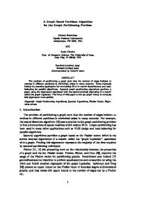
Definition 2.4 Let G = (V, E) be any graph, and J ⊆ V any subset of its vertices. We denote by outG (J) = EG (J, V \ J), and we call the edges in outG (J) the terminal edges for J. For each terminal edge e = (u, v), with u ∈ J, v 6∈ J, we call u the interface vertex and v the terminal vertex for J. We denote by ΓG (J) and TG (J) the sets of all interface and terminal vertices for J, respectively, and we omit the subscript G when clear from context (see Figure 2.1).
J Γ(J)
out(J) T (J) Figure 2.1: Terminal edges, and terminal and interface vertices for set J.
Definition 2.5 Given a graph G, a subset J of its vertices, and a parameter α > 0, we say that J is α-well-linked, iff for any partition (J1 , J2 ) of J, if we denote by T1 = out(J1 ) ∩ out(J), and by T2 = out(J2 ) ∩ out(J), then |E(J1 , J2 )| ≥ α · min {|T1 |, |T2 |} Notice that if G is a connected graph and J ⊂ V (G) is α-well-linked for any α > 0, then G[J] must be connected. Finally, we define ρ-balanced α-well-linked bi-partitions. Definition 2.6 Let G be any graph, and let ρ > 1, 0 < α ≤ 1 be any parameters. We say that a bi-partition (S, S) of V (G) is ρ-balanced and α-well-linked, iff |S|, |S| ≥ |V (G)|/ρ and both S and S are α-well-linked.
2.3
Canonical Vertex Sets and Solutions
As already mentioned in the Introduction, we will perform a number of graph contraction steps on the input graph G, where in each such graph contraction step, a sub-graph of G will be replaced with a grid. So in general, if H is the current graph, we will also be given a collection Z of disjoint subsets of vertices of H, such that for each Z ∈ Z, H[Z] is the kZ × kZ grid, for some kZ ≥ 2. We will also ensure that ΓH (Z) is precisely the set of the vertices in the first row of the grid H[Z], and the edges in outH (Z) form a
matching between ΓH (Z) and TH (Z). Given such a graph H, and a collection Z of vertex subsets, we will be looking for solutions in which the edges of the grids H[Z] do not participate in any crossings. This motivates the following definitions of canonical vertex sets and canonical solutions. Assume that we are given a graph G and a collection Z of disjoint subsets of vertices of G, (but some vertices of G may not belong to any subset Z ∈ Z).
property (P2) iff there is a planar drawing of J in which all interface vertices Γ(J) lie on the boundary of the same face, that we refer to as the outer face. We denote such a planar drawing by π(J). If there are several such drawing, we select any of them arbitrarily.
Definition 2.7 We say that a subset J ⊆ V of vertices is canonical for Z iff for each Z ∈ Z, either Z ⊆ J, or Z ∩ J = ∅.
Theorem 2.5 Suppose we are given any graph G = (V, E), a subset J ⊆ V of vertices, and a collection Z of disjoint subsets of vertices of V , such that each set Z ∈ Z is 1well-linked. Then we can efficiently find a partition J of J, such that each set J 0 ∈ JPis α∗ -well linked for α∗ = Ω(1/(log3/2 n log log n)), and J 0 ∈J | out(J 0 )| ≤ 2| out(J)|. Moreover, if J has any combination of the following three properties: (1) property (P1); (2) property (P2); (3) it is a canonical set for Z, then each set J 0 ∈ J will also have the same combination of these properties.
We next define canonical drawings and canonical solutions w.r.t. the collection Z of subsets of vertices: Definition 2.8 Let G = (V, E) be any graph, and Z any collection of disjoint subsets of vertices of G. We say that a drawing ϕ of G is canonical for Z iff for each Z ∈ Z, no edge of G[Z] participates in crossings. Similarly, we say that a solution E ∗ to the Minimum Planarization problem on G is canonical for Z, iff for each Z ∈ Z, no edge of G[Z] belongs to E ∗ . Definition 2.9 Given a graph G, a simple cycle X ⊆ G (that may be empty), and a collection Z of disjoint subsets of vertices of G, a strong solution to problem`π(G, S X, Z) is a ´ drawing ψ of G, in which the edges of E(X)∪ Z∈Z E(G[Z]) do not participate in any crossings, and G is embedded inside the bounding box X. The cost of the solution is the number of edge crossings in ψ. A weak solution to problem π(G, X, Z) is a subset E 0 ⊆ E(G) \ E(X) of edges, such that graph G \ E 0 has a planar drawing inside the bounding box X, and for all Z ∈ Z, E 0 ∩ E(G[Z]) = ∅. We will sometimes use the above definition for problem π(G0 , X, Z), where G0 is a sub-graph of G. That is, some sets Z ∈ Z may not be contained in G0 , or only partially contained in it. We can then define Z 0 to contain, for each Z ∈ Z, the set Z ∩ V (G0 ). We will sometimes use the notion of weak or strong solution to problem π(G0 , X, Z) to mean weak or strong solutions to π(G0 , X, Z 0 ), to simplify notation.
2.4
Well-linked Decompositions
The next theorem summarizes well-linked decomposition of graphs, which has been used extensively in graph decomposition (e.g., see [7, 26]). Theorem 2.4 (Well-linked decomposition) Given any graph G = (V, E), and any subset J ⊆ V of vertices, we can efficiently find a partition J of J, such that each set J 0 ∈P J is α∗ -well-linked for α∗ = Ω(1/(log3/2 n log log n)), and J 0 ∈J | out(J 0 )| ≤ 2| out(J)|. We now define some additional properties that set J may possess, that we use throughout the paper. We will then show that if a set J has any collection of these properties, then we can find a well-linked decomposition J of J, such that every set J 0 ∈ J has these properties as well. Definition 2.10 Given a graph G and any subset J ⊆ V (G) of its vertices, we say that J has property (P1) iff the vertices of T (J) are connected in G \ J. We say that it has
The next theorem is an extension of Theorem 2.4, and its proof is omitted due to lack of space.
Throughout the paper, we use α∗ to denote the parameter from Theorem 2.5.
3.
HIGH LEVEL ALGORITHM OVERVIEW
In this section we provide a high-level overview of the algorithm. We start by defining the notion of nasty vertex sets. Definition 3.1 Given a graph G, we say that a subset S ⊆ V (G) of vertices is nasty iff it has properties (P1) and (P2), 216 ·d6
· |Γ(S)|2 , where α∗ is the parameter from and |S| ≥ (α∗max )2 Theorem 2.5. Note that we do not require that G[S] is connected. For the sake of clarity, let us first assume that the input graph G contains no nasty sets. Fix any optimal drawing ϕ of G. An edge of G is called good iff it does not participate in any crossings in ϕ. Our algorithm then proceeds as follows. We use a balancing parameter ρ = O(OPTcr (G) · poly(dmax · log n)) whose exact value is set later. The algorithm has O(ρ · log n) iterations. At the beginning of each iteration h, we are given a collection G1 , . . . , Gkh of kh ≤ OPTcr (G) subgraphs of G, together with bounding boxes Xi ⊆ Gi for all i. The graphs Gi are completely disjoint, except that they may share vertices or edges that belong to their bounding boxes. We are also guaranteed that w.h.p., there is a strong solution to each problem π(Gi , Xi ), of total cost at most OPTcr (G). In the first iteration, k1 = 1, and the only graph is G1 = G, whose bounding box is X0 = ∅. We now proceed to describe each iteration. The idea is to find a skeleton Ki for each graph Gi , with Xi ⊆ Ki , such that Ki only contains good edges — that is, edges that do not participate in any crossings in the fixed optimal solution ϕ, and Ki has a unique planar drawing, in which Xi serves as the bounding box. Therefore, we can efficiently find the drawing ϕKi of the skeleton Ki , induced by the optimal drawing ϕ. We then decompose the remaining graph Gi \E(Ki ) into clusters, by removing a small subset of edges from it, so that, on the one hand, for each such cluster C, we know the face FC of ϕKi where we should embed it, while on the other hand, different clusters C, C 0 do not interfere with each other, in the sense that we can find an embedding
of each one of these clusters separately, and their embeddings do not affect each other. For each such cluster C, we then define a new problem π(C, γ(FC )), where γ(FC ) is the boundary of the face FC . We will ensure that all resulting sub-problems have strong solutions whose total cost is at most OPTcr (G). In particular, there are at most OPTcr (G) resulting sub-problems, for which ∅ is not a feasible weak solution. Therefore, in the next iteration we will need to solve at most OPTcr (G) new sub-problems. The main challenge is to find, for each graph Gi , a skeleton Ki , such that the number of vertices in each resulting cluster C is bounded by roughly (1 − 1/ρ)|V (Gi )|, so that the number of iterations is indeed bounded by O(ρ log n). We need this bound on the number of iterations, since the probability of successfully constructing the skeletons in each iteration is only (1 − 1/ρ). Roughly speaking, we are able to build the skeleton as required, if we can find a ρ-balanced α-well-linked bipartition of the vertices of Gi , where α = 1/ poly(dmax ·log n). We are only able to find such a partition if no nasty sets exist in G. More precisely, we show an efficient algorithm, that either finds the desired bi-partition, or returns a nasty vertex set. In order to obtain the whole algorithm, we therefore need to deal with nasty sets. We do so by performing a graph contraction step, which is formally defined in the next section. Informally, given a nasty set S, we find a partition X of S, such that for every pair X, X 0 ∈ X , the graphs G[X], G[X 0 ] share at most one vertex, and no edges. The unique vertex v ∈ X ∩ X 0 must belong to the interface of ∗ both X and X 0 . Each such set X Pis also α -well-linked, has properties (P1) and (P2), and |Γ(X)| ≤ O(|Γ(S)|). X∈X We then replace each sub-graph G[X] of G by a grid ZX , whose interface is Γ(X). After we do so for each X ∈ X , we denote by G|S the resulting contracted graph. Notice that we have replaced G[S] by a much smaller graph, whose size is bounded by O(|Γ(S)|2 ). Let Z denote the collection of sets V (ZX ) of vertices, for X ∈ X . We then show that the cost of the optimal solution to problem π(G|S , ∅, Z) is at most poly(dmax · log n)OPTcr (G). Therefore, we can restrict our attention to canonical solutions only. We also show that it is enough to find a weak solution to problem π(G|S , ∅, Z), in order to obtain a weak solution for the whole graph G. Unfortunately, we do not know how to find a nasty set S, such that the corresponding contracted graph G|S contains no nasty sets. Instead, we do the following. Let H = G|S be the current graph, which is a result of the graph contraction step on some set S of vertices, and let Z be the corresponding collection of sub-sets of vertices representing the grids. Suppose we can find a nasty canonical set R in the graph H. We show that this allows us to find a new set S 0 of vertices in G, such that the contracted graph G|S 0 contains fewer vertices than G|S . Returning to our algorithm, let G|S be the current contracted graph. We show that with high probability, the algorithm either returns a weak ´solution for G|S of cost ` O (OPTcr (G))5 poly(dmax · log n) , or it returns a nasty canonical subset S 0 of G|S . In the former case, we can recover a good weak solution for the original graph G. In the latter case, we find a subset S 00 of vertices in the original graph G, and perform another contraction step on G, obtaining a new graph G|S 00 , whose size is strictly smaller than that of G|S . We then apply the algorithm to graph G|S 00 . Since the total number of graph contraction steps is bounded by n, after n such iterations, we are guaranteed w.h.p. to obtain a weak
` ´ feasible solution of cost O (OPTcr (G))5 poly(dmax · log n) to π(G, ∅), thus satisfying the requirements of Theorem 1.3. We now turn to formal description of the algorithm. One of the main ingredients is the graph contraction step, summarized in the next section.
4.
GRAPH CONTRACTION STEP
The input to the graph contraction step consists of the input graph G, and a subset S ⊆ V (G) of vertices, for which properties (P1) and (P2) hold. It will be convenient to think of S as a nasty set, but we do not require it. Let C = {G1 , . . . , Gq } be the set of all connected components of G[S]. For each 1 ≤ i ≤ q, let Γi = V (Gi ) ∩ Γ(S) = Γ(V (Gi )) be the set of the interface vertices of Gi . The goal of the graph contraction step is to find, for each 1 ≤ i ≤ q, a partition Xi ofS the set V (Gi ), that has the following properties. Let X = qi=1 Xi . C1. Each set X ∈ X is α∗ -well-linked, and has properties (P1) and (P2). Moreover, there is a planar drawing π 0 (X) of G[X], and a simple closed curve γX , such that G[X] is embedded inside γX in π 0 (X), and the vertices of Γ(X) lie on γX . C2. For each X ∈ X , either |Γ(X)| = 2, or there is a ∗ ∗ ] is , R1 , . . . , Rt ) of X, such that G[CX partition (CX ∗ 2-connected and Γ(X) ⊆ CX . Moreover, for each 1 ≤ ∗ t0 ≤ t, there is a vertex ut0 ∈ CX , whose removal from G[X] separates the vertices of Rt0 from the remaining vertices of X. C3. For each pair X, X 0 ∈ X , the two sets of vertices are completely disjoint, except for possibly sharing one interface vertex, v ∈ Γ(X) ∩ Γ(X 0 ). S C4. For each 1 ≤ i ≤ q, if Γ0i = X∈Xi Γ(X), then |Γ0i | ≤ 9|Γi |. C5. For each X ∈ X , |X| ≥ (α∗ |Γ(X)|)2 /64d2max . 0 , that For each set X ∈ X , we now define a new graph ZX will eventually replace the sub-graph G[X] in G. Intuitively, 0 we need ZX to contain the vertices of Γ(X) and to be 1well-linked w.r.t. these vertices. We also need it to have a unique planar embedding where the vertices of Γ(X) lie on the boundary of the same face, and finally, we need the 0 size of the graph ZX to be relatively small, since this is a graph contraction step. The simplest graph satisfying these properties is a grid of size |Γ(X)| × |Γ(X)|. Specifically, we first define a graph ZX as follows: if |ΓX | = 1, then ZX consists of a single vertex, and if |ΓX | = 2, then ZX consists of a single edge. Otherwise, ZX is a grid of size 0 |Γ(X)| × |Γ(X)|. In order to obtain the graph ZX , we add the set Γ(X) of vertices to ZX , and add a matching between the vertices of the first row of the grid and the vertices of Γ(X). This is done so that the order of the vertices of Γ(X) along the first row of the grid is the same as their order along the curve γX in the drawing π 0 (X). We refer to these new edges as the matching edges. For the cases where |ΓX | = 1 0 and |ΓX | = 2, we obtain ZX by adding the vertices of Γ(X) to ZX , and adding an arbitrary matching between ΓX and the vertices of ZX . (See Figure 4.1). The contracted graph G|S is obtained from G, by replacing, for each X ∈ X , the subgraph G[X] of G, with the
Therefore, if the initial vertex set S is nasty, then we have indeed reduced the graph size, as |V (H)| < |V (G)|. We now define a collection Z of subsets of vertices of H, as follows: Z = {V (ZX ) | X ∈ X }. Notice that these sets are completely disjoint, as ZX does not contain the interface vertices Γ(X). Moreover, for each Z ∈ Z, H[Z] is a grid, ΓH (Z) consists of the vertices in the first row of the grid, and outH (Z) consists of the set of the matching edges, each of which connects a vertex in the first row of the grid Z to a distinct vertex in TH (Z). Using Definitions 2.7 and 2.8, we can now define canonical subsets of vertices, canonical drawings and canonical solutions to the Minimum Planarization problem on H, with respect to Z. Our main result for graph contraction is summarized in the next theorem, whose proof is omitted due to lack of space.
...
vp
πX v1 v2
v3
...
! ZX
v1 v2 v3
...
Theorem 4.1 Let S ⊆ V (G) be any subset of vertices with properties (P1) and (P2), and let {G1 , . . . , Gq } be the set of all connected components of graph G[S]. Then for each 1 ≤ i ≤ q, we can efficiently find a partition Xi of V (Gi ), S such that the resulting partition X = qi=1 Xi of S has properties (C1)–(C5). Moreover, there is a canonical drawing of the resulting contracted graph H = G|S with O(d9max ·log10 n· (log log n)4 · OPTcr (G)) crossings.
vp
(a) General case
πX v1
πX
πX
v1
v1
! ZX u1
πX
v1
v2
! ZX
! ZX u1
u1
u2 u1
v1 v2
v1 (b) |Γ(X)| = 1
v1
The next claim shows, that in order to find a good solution to the Minimum Planarization problem on G, it is enough to solve it on G|S .
v2
! ZX
u2
v1 v2
(c) |Γ(X)| = 2
0 . Figure 4.1: Graph ZX
0 graph ZX . This is done as follows: first, delete all vertices and edges of G[X], except for the vertices of Γ(X), from G, 0 and add the edges and the vertices of ZX instead. Next, identify the copies of the interface vertices Γ[X] in the two graphs. Let H = G|S denote the resulting contracted graph. Notice that
q X X
0 |V (ZX )| ≤
i=1 X∈Xi
q X X
2|Γ(X)|2
i=1 X∈Xi
≤
q X
2|Γ0i |2 d2max
(4.1)
i=1
≤ 162d2max |Γ|2 (we have used the fact that a vertex may belong to the interface of at most dmax sets X ∈ Xi , and Property (C4)).
Claim 4.2 Let S be any subset of vertices of G, X any partition of S with properties (C1)–(C5), H = G|S the corresponding contracted graph and Z the collection of grids ZX for X ∈ X . Then given any canonical solution E ∗ to the Minimum Planarization problem on H, we can efficiently find a solution of cost O(dmax )|E ∗ | to Minimum Planarization on G. Proof. Partition set E ∗ of edges into two subsets: E1∗ 0 for X ∈ X , contains all edges that belong to sub-graphs ZX ∗ and E2 contains all remaining edges. Notice that since E ∗ is a canonical solution, each edge e ∈ E1∗ must be a matching 0 . Also from the construction of the edge for some graph ZX contracted graph H, all edges in E2∗ belong to E(G). Consider some set X ∈ X , and let Γ0 (X) ⊆ Γ(X) denote 0 , whose matching the subset of the interface vertices of ZX S edges belong to E1∗ . Let Γ0 = X∈X Γ0 (X). We now define a subset E1∗∗ of edges of G as follows: for each vertex v ∈ Γ0 , add all edges incident to v in G to E1∗∗ . Finally, we set E ∗∗ = E1∗∗ ∪ E2∗ . Notice that E ∗∗ is a subset of edges of G, and |E ∗∗ | = |E1∗∗ | + |E2∗ | ≤ dmax |E1∗ | + |E2∗ | ≤ dmax |E ∗ |. In order to complete the proof of the claim, it is enough to show that E ∗∗ is a feasible solution to the Minimum Planarization problem on G. Let G0 = G \ E ∗∗ , let H 0 = H \ E ∗ , and let ψ be a planar drawing of H 0 . It is now enough to construct a planar drawing ψ 0 of G0 . In order to do so, we start from the planar drawing ψ of H 0 . We then consider the sets X ∈ X one-by0 one. For each such set, we replace the drawing of ZX \Γ0 (X) with a drawing of G[X]\Γ0 (X). The drawings of the vertices in Γ(X) are not changed by this procedure. After all sets X ∈ X are processed, we will obtain a planar drawing of graph G0 (that may also contain drawings of some edges in E ∗∗ , that we can simply erase).
Consider some such set X ∈ X . Let G be the current graph (obtained from H 0 after a number of such replacement steps), and let ψ be the current planar drawing of G. Observe that the grid ZX has a unique planar drawing. We 0 say that a planar drawing of graph ZX \ Γ0 (X) is standard 0 in ψ, iff we can draw a simple closed curve γX , such that 0 ZX is embedded completely inside γX ; no other vertices or 0 0 edges of G are embedded inside γX ; the only edges that γX 0 intersects are the matching edges of ZX \ Γ0 (X), and each 0 such matching edge is intersected exactly once by γX . 0 0 It is possible that the drawing of ZX \ Γ (X) in ψ is not standard. However, since ψ is planar, this can only happen for the following three reasons: (1) some connected component C of the current graph G is embedded inside some face of the grid ZX : in this case we can simply move the drawing of C elsewhere; (2) there is some subset C of V (G), and a vertex v ∈ Γ(X) \ Γ0 (X), such that ΓG (C) = v, and G[C] is embedded inside one of the faces of the grid ZX incident to the other endpoint of the matching edge of v; and (3) there is some subset C of V (G), and two consecutive vertices u, v ∈ Γ(X) \ Γ0 (X), such that ΓG (C) = {u, v}, and G[C] is embedded inside the unique face of the grid ZX incident to the other endpoints of the matching edges of u and v. In the latter two cases, we simply move the drawing of C right outside the grid, so that the corresponding matching edges now cross the curve γ 0 (X). To summarize, we can transform the current planar draw˜ such ing ψ of the graph G into another planar drawing ψ, 0 0 that the induced drawing of ZX \ Γ (X) is standard. We can 0 \Γ0 (X) now draw a simple closed curve γ 00 (X), such that ZX 00 is embedded inside γ (X), no other vertices or edges are embedded inside γ 00 (X), and the set of vertices whose drawings lie on γ 00 (X) is precisely Γ(X) \ Γ0 (X). Notice that the ordering of the vertices of Γ(X) \ Γ0 (X) along this curve is exactly the same as their ordering along the curve γ(X) in the planar embedding π 0 (X) of G[X], guaranteed by Property (C1). Let π 00 (X) be the drawing of G[X] \ Γ0 (X) induced by π 0 (X). We can now simply replace the drawing 0 \ Γ0 (X) with the drawing π 00 (X) of G[X] \ Γ0 (X), of ZX 00 , and the drawings of the identifying the curves γX and γX 0 vertices in Γ(X) \ Γ (X) on them. The resulting drawing remains planar, and the drawings of the vertices in Γ(X) do not change. Finally, we show that if we find a nasty canonical set in G|S , then we can contract G even further. The proof of the following theorem is omitted due to lack of space. Theorem 4.3 Let S be any subset of vertices of G, X any partition of S with properties (C1)–(C5), H = G|S the corresponding contracted graph, and Z the corresponding collection of grids ZX for X ∈ X . Then given any nasty canonical vertex set R ⊆ V (H), we can efficiently find a subset S 0 ⊆ V (G) of vertices, and a partition X 0 of S 0 , such that properties (C1)–(C5) hold for X 0 , and if H 0 = G|S 0 is the corresponding contracted graph, then |V (H 0 )| < |V (H)|. Moreover, there is a canonical drawing ϕ0 of H 0 with crϕ0 (H 0 ) = O(d9max · log10 n · (log log n)4 · OPTcr (G)). Notice that Claim 4.2 applies to the new contracted graph as well.
5.
THE ALGORITHM
The algorithm consists of a number of stages. In each stage j, we are given as input a subset S of vertices of G, the contracted graph H = G|S , and the collection Z of disjoint sub-sets of vertices of H, corresponding to the grids ZX obtained during the contraction step. The goal of stage j is to either produce a nasty canonical set R in H, or to find a weak feasible solution to problem π(H, ∅, Z). We prove the following theorem. Theorem 5.1 There is an efficient randomized algorithm, that, given a contracted graph H, a corresponding collection Z of disjoint subsets of vertices of H, and a bound OPT0 on the cost of the strong optimal solution to problem π(H, ∅, Z), with probability at least 1/ poly(n), produces either a nasty canonical subset R of vertices of H, or a weak feasible solution E ∗ , |E ∗ | ≤ O((OPT0 )5 poly(dmax · log n)) for problem π(H, ∅, Z). (Here, n = |V (G)|). We provide a high-level sketch of the proof of this theorem in the rest of this section, but we first show that Theorems 1.3, 1.1 and Corollary 1.1 follow from it. We start with proving Theorem 1.3, by showing an efficient randomized algorithm to find a subset E ∗ ⊆ E(G) of edges, such that G\E ∗ is planar, and |E ∗ | ≤ O((OPTcr (G))5 ·poly(dmax · log n)). We assume that we know the value OPTcr (G), by using the standard practice of guessing this value, running the algorithm, and then adjusting the guessed value accordingly. It is enough to ensure that whenever the guessed value OPT ≥ OPTcr (G), the algorithm indeed returns a subset E ∗ of edges, |E ∗ | ≤ O(OPT5 poly(dmax ·log n)), such that G\E ∗ is a planar graph w.h.p. Therefore, from now on we assume that we are given a value OPT ≥ OPTcr (G). The algorithm consists of a number of stages. The input to stage j is a contracted graph H, with the corresponding family Z of vertex sets. In the input to the first stage, H = G, and Z = ∅. In each stage j, we run the algorithm from Theorem 5.1 on the current contracted graph H, and the family Z of vertex subsets. From Theorem 4.1, there is a strong feasible solution to problem π(H, ∅, Z) of cost O(OPT · poly(log n · dmax )), and so we can set the parameter OPT0 to this value. Whenever the algorithm returns a nasty canonical set R in graph H, we terminate the current stage, and compute a new contracted graph H0 , guaranteed by Theorem 4.3. Graph H0 , together with the corresponding family Z 0 of vertex subsets, becomes the input to the next stage. Alternatively, if, after poly(n) executions of the algorithm from Theorem 5.1, no nasty canonical set is returned, then with high probability, one of the algorithm executions has returned a weak feasible solution E ∗ , |E ∗ | ≤ O(OPT5 poly(dmax · log n)) for problem π(H, ∅, Z). From Claim 4.2, we can recover from this solution a planarizing set E ∗∗ of edges for graph G, with |E ∗∗ | = O(OPT5 poly(dmax · log n)). Since the size of the contracted graph H goes down after each contraction step, the number of stages is bounded by n, thus implying Theorem 1.3. Combining Theorem 1.3 with Theorem 1.2 immediately gives Theorem 1.1. Finally, we obtain Corollary 1.1 as follows. Recall that the algorithm of Even et al. [10] computes a drawing of any n-vertex bounded degree graph G with O(log2 n)·(n+OPTcr (G)) crossings. It was shown in [9], that this algorithm can be extended to arbitrary graphs, where the number of crossings becomes O(poly(dmax )·log2 n)·(n+ OPTcr (G)). We run their algorithm, and the algorithm pre-
sented in this section, on graph G, and output the better of the two solutions. If OPTcr (G) < n1/10 , then our algorithm gives an O(n9/10 poly(dmax · log n))-approximation; otherwise, the algorithm of [10] gives an O(n9/10 poly(dmax · log n))-approximation. The remainder of this section is devoted to proving Theorem 5.1. Recall that we are given the contracted graph H, and a collection Z of vertex-disjoint subsets of V (H). For each Z ∈ Z, H[Z] is a grid, and E(Z, V (H) \ Z) consists of a set MZ of matching edges. Each such edge connects a vertex in the first row of Z to a distinct vertex in TH (Z), and these edges form a matching between the first row of Z and TH (Z). Abusing the notation, we denote the bound on the cost of the strong optimal solution to π(H, ∅, Z) by OPT from now on, and the number of vertices in H by n. For each Z ∈ Z, we use Z to denote both the set of vertices itself, and the grid H[Z]. We assume √ throughout the rest of the section that OPT · d6max < n: otherwise, √ if OPT · d6max ≥ n, then the set E 0 of all edges of H that do not participate in grids Z ∈ Z, is a feasible weak canonical solution for problem π(H, ∅, Z). It is easy to see that |E 0 | ≤ O(OPT2 poly(dmax )): this is clearly the case if |E 0 | ≤ 4n; otherwise, if |E 0 | > 4n, then by Theorem 2.3, OPT = Ω(n), and so |E 0 | = O(n2 ) = O(OPT2 ). We use two parameters: ρ = O(OPT poly(dmax · log n)) and m∗ = O(OPT3 · poly(dmax · log n)). The algorithm consists of 2ρ log n iterations. The input to iteration h is a collection G1 , . . . , Gkh of kh ≤ OPT sub-graphs of H, together with bounding boxes Xi ⊆ Gi for all 1 ≤ i ≤ kh . We denote Hi = Gi \ V (Xi ) and n(Hi ) = |V (Hi )|. Additionally, we have collections E (1) , . . . , E (h−1) of edges of H, 0 where for each 1 ≤ h0 ≤ h − 1, set E (h ) has been com0 puted in iteration h . We say that (G1 , X1 ), . . . , (Gkh , Xkh ), and E (1) , . . . , E (h−1) is a valid input to iteration h, iff the following invariants hold: V1. For all 1 ≤ i, j ≤ kh , graphs Hi and Hj are completely disjoint. V2. For all 1 ≤ i ≤ kh , Gi ⊆ H\(E (1) , . . . , E (h−1) ), and Hi is the sub-graph of H induced by V (Hi ). In particular, no edges e ⊆ V (Hi ) belong to E (1) , . . . , E (h−1) . MoreS 0 over, every edge e ∈ E(H) belongs to either hh0 =1 E (h ) Skh or to i=1 Gi . V3. For all Z ∈ Z, for all 1 ≤ i ≤ kh , either Z ∩V (Hi ) = ∅, or Z ⊆ V (Hi ). Let Zi = {Z ∈ Z | Z ⊆ V (Hi )}. V4. For each 1 ≤ i ≤ kP h , there is a strong solution ϕi to h π(Gi , Xi , Zi ), with ki=1 crϕi (Gi ) ≤ OPT. V5. If we are given, for each 1 ≤ i ≤ kh , any weak solu˜ (h) = tion E 0 to problem π(Gi , Xi , Zi ), and denote E Skh i (1) (h−1) (h) ˜ ∪· · · E ∪E is a feasible weak i=1 Ei , then E solution to problem π(H, ∅, Z). V6. For each 1 ≤ h0 < h, and 1 ≤ i ≤ kh , the number of 0 edges in E (h ) incident on vertices of Hi is at most m∗ , 0 and |E (h ) | ≤ OPT · m∗ . Moreover, no edges in grids S (h0 ) Z ∈ Z belong to h−1 . h0 =1 E V7. Let nh = (1 − 1/ρ)(h−1)/2 · n. For each 1 ≤ i ≤ kh , either n(Hi ) ≤ nh , or Xi = ∅ and n(Hi ) ≤ nh−1 .
The input to the first iteration consists of a single graph, G1 = H, with the bounding box X1 = ∅. It is easy to see that all invariants hold for this input. We end the algorithm at iteration h∗ , where nh∗ ≤ (m∗ · ρ · log n)2 . Clearly, h∗ ≤ 2ρ log n, from Invariant (V7). Let G be the set of all instances that serve as input to iteration h∗ . We need the following theorem, whose proof is omitted due to lack of space. Theorem 5.2 There is an efficient algorithm, that, given any problem instance π(G, X, Z 0 ), where V (G \ X) is canonical for Z 0 , and π(G, X, Z 0 ) has a strong solution of cost OPT, finds a weak feasible solution to π(G, X, Z 0 ) of cost √ 3 O(OPT · n0 · poly(dmax · log n0 ) + OPT ), where n0 = |V (G \ X)|, and dmax is the maximum degree in G. (h∗ )
For each 1 ≤ i ≤ kh∗ , let Ei be the weak solution from Skh∗ (h∗ ) ∗ Theorem 5.2, and let E (h ) = i=1 Ei . Let OPTi denote the cost of the strong optimal solution to π(Gi , Xi , Zi ). p Pkh∗ ∗ Then |E (h ) | = i=1 O(OPTi · n(Hi ) · poly(dmax · log n) + 3 OPTi ). Since n(Hi ) ≤ nh∗ −1 ≤ 2nh∗ for all i, this is Pkh∗ O(OPTi ·m∗ ·ρ·poly(dmax log n)+OPT3i ) ≤ bounded by i=1 Pkh∗ ∗ O(OPT · m · ρ · poly(dmax log n) + OPT3 ), as i=1 OPTi ≤ S ∗ OPT from Invariant (V4). The final solution is E ∗ = hh=1 E (h) , and
∗
|E | ≤
∗ hX −1
∗
|E (h) | + |E (h ) |
h=1
≤ (2ρ log n)(OPT · m∗ ) + O(OPT · m∗ · ρ · poly(dmax · log n)) + O(OPT3 ) = O(OPT5 poly(dmax · log n)). We say that the execution of iteration h is successful, iff it either produces a valid input to the next iteration, together with the set E (h) of edges, or finds a nasty canonical set in H. We can execute each iteration, so that it is successful with probability at least (1 − 1/ρ), if all previous iterations were successful. If any iteration returns a nasty canonical set, then we stop the algorithm and return this vertex set as an output. Since there are at most 2ρ log n iterations, the probability that all iterations are successful is at least (1 − 1/ρ)2ρ log n ≥ 1/ poly(n). In order to complete the proof of Theorem 5.1, it is now enough to show an algorithm for executing each iteration, such that, given a valid input to the current iteration, the algorithm either finds a nasty canonical set in H, or returns a valid input to the next iteration, with probability at least ρ1 . Due to lack of space, this part is omitted, and can be found in the full version of the paper, available as an arXiv report, arXiv:1012.0255v1.
6.
CONCLUSIONS
We have shown an efficient randomized algorithm to find a drawing of any graph G` in the plane, with the number of ´ crossings bounded by O (OPTcr (G))10 poly(dmax · log n) . We did not make an effort to optimize the powers of OPT, dmax and log n in this guarantee, or the constant hidden in the O(·) notation, and we believe that they can be improved. We hope that the technical tools developed in this
paper will help obtain better algorithms for the Minimum Crossing Number problem. A specific possible direction is obtaining efficient algorithms for ρ-balanced α-well-linked bi-partitions. In particular, an interesting open question is whether there is an efficient algorithm, that, given an n-vertex graph G with maximum degree dmax , finds a ρbalanced α-well-linked bi-partition of G, for values ρ, 1/α = poly(dmax · log n). In fact it is not even clear whether such a bi-partition exists in every graph. We note that the dependence of ρ on dmax is necessary, for example, in the star graph. This question appears to be interesting in its own right, and its positive resolution (even if the parameters ρ and α depend on OPTcr (G)) would greatly simplify our algorithm and improve its performance guarantee.
[11] M. R. Garey and D. S. Johnson. Crossing number is NP-complete. SIAM J. Algebraic Discrete Methods, 4(3):312–316, 1983. [12] I. Gitler, P. Hlinˇen´ y, J. Lea˜ nos, and G. Salazar. The crossing number of a projective graph is quadratic in the face-width. Electronic Notes in Discrete Mathematics, 29:219–223, 2007. [13] M. Grohe. Computing crossing numbers in quadratic time. J. Comput. Syst. Sci., 68(2):285–302, 2004. [14] R. Guy. A combinatorial problem. Nabla (Bulletin of the Malayan Mathematical Society), 7:68–72, 1960. [15] P. Hlinen´ y. Crossing number is hard for cubic graphs. J. Comb. Theory, Ser. B, 96(4):455–471, 2006. [16] P. Hlinˇen´ y and M. Chimani. Approximating the crossing number of graphs embeddable in any Acknowledgements. orientable surface. In Proc. 21st Annual ACM-SIAM The author thanks Yury Makarychev and Anastasios SidiropouSymposium on Discrete Algorithms, 2010. los for many fruitful discussions, and for reading earlier [17] P. Hlinˇen´ y and G. Salazar. Approximating the drafts of the paper. crossing number of toroidal graphs. Lecture Notes in Computer Science, 4835/2007:148–159, 2007. [18] J. Hopcroft and R. Tarjan. Efficient planarity testing. 7. REFERENCES J. ACM, 21(4):549–568, 1974. [1] M. Ajtai, V. Chv´ atal, M. Newborn, and E. Szemer´edi. [19] K. Kawarabayashi and B. A. Reed. Computing Crossing-free subgraphs. Theory and Practice of crossing number in linear time. In STOC, pages Combinatorics, pages 9–12, 1982. 382–390, 2007. [2] C. Ambuhl, M. Mastrolilli, and O. Svensson. [20] F. T. Leighton. Complexity issues in VLSI: optimal Inapproximability results for sparsest cut, optimal layouts for the shuffle-exchange graph and other linear arrangement, and precedence constrained networks. MIT Press, 1983. scheduling. In Proceedings of the 48th Annual IEEE [21] F. T. Leighton and S. Rao. Multicommodity max-flow Symposium on Foundations of Computer Science, min-cut theorems and their use in designing pages 329–337, 2007. approximation algorithms. Journal of the ACM, [3] S. Arora, S. Rao, and U. V. Vazirani. Expander flows, 46:787–832, 1999. geometric embeddings and graph partitioning. J. [22] R. J. Lipton and R. E. Tarjan. A separator theorem ACM, 56(2), 2009. for planar graphs. SIAM Journal on Applied [4] S. N. Bhatt and F. T. Leighton. A framework for Mathematics, 36(2):177–189, 1979. solving VLSI graph layout problems. [23] J. Matouˇsek. Lectures on discrete geometry. J. Comput. Syst. Sci., 28(2):300–343, 1984. Springer-Verlag, 2002. [5] K. J. B¨ or¨ ozky, J. Pach, and G. T´ oth. Planar crossing [24] J. Pach and G. T´ oth. Thirteen problems on crossing numbers of graphs embeddable in another surface. numbers. Geombinatorics, 9(4):194–207, 2000. Int. J. Found. Comput. Sci., 17(5):1005–1016, 2006. [25] S. Pan and R. B. Richter. The crossing number of K11 [6] S. Cabello and B. Mohar. Adding one edge to planar is 100. J. Graph Theory, 56(2):128–134, 2007. graphs makes crossing number hard. In Proc. ACM [26] H. R¨ acke. Minimizing congestion in general networks. Symp. on Computational Geometry, 2010. In In Proceedings of the 43rd IEEE Symposium on [7] C. Chekuri, S. Khanna, and F. B. Shepherd. Foundations of Computer Science (FOCS), pages Multicommodity flow, well-linked terminals, and 43–52, 2002. routing problems. In STOC ’05: Proceedings of the [27] R. B. Richter and G. Salazar. Crossing numbers. In thirty-seventh annual ACM symposium on Theory of L. W. Beineke and R. J. Wilson, editors, Topics in computing, pages 183–192, New York, NY, USA, 2005. Topological Graph Theory, chapter 7, pages 133–150. ACM. Cambridge University Press, 2009. [8] M. Chimani, P. Hlinˇen´ y, and P. Mutzel. [28] L. A. Szekely. Progress on crossing number problems. Approximating the crossing number of apex graphs. In In SOFSEM, pages 53–61, 2005. Graph Drawing, pages 432–434, 2008. [29] P. Tur´ an. A note of welcome. J. Graph Theory, 1:1–5, [9] J. Chuzhoy, Y. Makarychev, and A. Sidiropoulos. On 1977. graph crossing number and edge planarization. [30] I. Vrto. Crossing numbers of graphs: A bibliography. Proceedings of the Twenty-Second Annual ACM-SIAM http://www.ifi.savba.sk/~imrich. Symposium on Discrete Algorithms (SODA), pages [31] H. Whitney. Congruent graphs and the connectivity of 1050–1069, 2011. Full version: arXiv:1010.3976v1, graphs. American Journal of Mathematics, Oct. 2010. 54(1):150–168, 1932. [10] G. Even, S. Guha, and B. Schieber. Improved [32] D. R. Wood and J. A. Telle. Planar decompositions approximations of crossings in graph drawings and and the crossing number of graphs with an excluded VLSI layout areas. SIAM J. Comput., 32(1):231–252, minor. New York J. Mathematics, 13:117–146, 2007. 2002.