An Algorithm for WSN Clock Synchronization: Uncertainty and Convergence Rate Trade Off. Daniele Fontanelli and Dario Petri. DISI â Department of ...
An Algorithm for WSN Clock Synchronization: Uncertainty and Convergence Rate Trade Off Daniele Fontanelli and Dario Petri DISI – Department of Engineering and Computer Science, University of Trento Via Sommarive, 14 – 38100, Trento, Italy Email: {fontanelli,petri}@disi.unitn.it
Abstract—Achieving tight time synchronization between wireless sensor network (WSN) nodes is essential to coordinate the activities of different devices. In this paper, a synchronization algorithm based on a linear controller is used to dynamically compensate both mutual offsets and drifts of the clock associated with the nodes of a WSN. This approach, compared with other existing solutions based on control theory, explicitly takes into account the inter–node communication latencies. Furthermore, it presents on optimal (fastest convergence) controller in the case of full visibility among nodes. In the case of noise in both the clock measurements and the clock drifts, a controller that reduces the noise effect on the synchronization accuracy is also proposed and compared to the optimal one. In all cases, the correct operation of the algorithm has been proved through simulations.
I. I NTRODUCTION The penetration of Wireless Sensor Networks (WSN) in a variety of applications, from robotics to factory automation, rises new and challenging sensing problems. For example, environmental surveillance is made more efficient wirelessly connecting a large number of distributed sensing devices. Locally measured data from each sensor are then post–processed together to obtain the overall picture of the system state and/or to act on it. The time in which the data is measured plays a fundamental role, as well as the accuracy of the measured phenomenon. Since the measurements are collected in each sensor node, the time stamp of each measurement is related to the local clock. Therefore, node clocks have to be synchronized to preserve the data meaning. Furthermore, synchronization protocols are also needed to coordinate the tasks running on different nodes of the network (for example, see [1]). Moreover, time synchronization is beneficial also to reduce the overall power consumption in those applications in which the network nodes should be active just for a limited fraction time. In fact, by synchronizing the wake–up and sleep times, unnecessary transmission, channel sensing and receiving attempts could be avoided. This paper proposes a distributed synchronization algorithm that cope with node clock offsets and drifts and stems from the theoretical framework proposed in [2]. This work was supported by the FP-7 EC under contract IST-2008-224428 “CHAT - Control of Heterogeneous Automation Systems” and “TRITon Trentino Research & Innovation for Tunnel Monitoring” financed by the Provincia Autonoma di Trento
The time synchronization problem is a well studied aspect of wireless networks, but it is still of great interest for scientists in the networking and measurement communities. Since WSN–specific synchronization protocols are mostly focused on the reduction of both computational burden and network traffic, at a reasonable price in terms of maximum achievable accuracy [3], general time protocols for measurement and control systems, as the well-known Precision Time Protocol (PTP) [4], are not very suitable for WSNs. Indeed, PTP frames are generally longer than the MAC-layer frames of the communication protocol IEEE 802.15.4 commonly used for the WSN radio modules [5] and, hence, it generates a considerable network overhead. WSN–specific synchronization protocols usually elects (or dynamically re–elects) a time reference node and transfers its local time to the other WSN nodes through multiple hops, while compensating the clock offsets between parent and child nodes [6]. A notable solution in which time information flow without any elected time reference node has been proposed by [7] using an effective nonlinear solution. Differently, a linear control algorithm is chosen in this paper to perform clock correction, in which clock times converge to a common network timescale on the basis of the time values collected from multiple nearby nodes. This idea is presented also in the Reference Broadcast Synchronization (RBS) protocol proposed by Elson in [8], that relies on a least–mean–square algorithm to estimate clock offsets and skews. A theoretical solution using an integral (PI) consensus controller has been proposed in [2], in which the controller has continuous knowledge of the time status of the other nodes, hence impractical due to unrealistic communication overhead. In this paper we propose an optimal (fastest convergence) PI-consensus control algorithm, based on [2], in order to work even when the time interval between two consecutive synchronization events is larger than the local timer resolution and change dynamically at run-time (due to node power savings approaches, as in [9]). On the other hand, we analyze the uncertainty of the synchronization algorithm due to both communication latencies and clock drift nuisances. Also the trade–off between the fastest controller and more accurate synchronization approaches is analyzed and validated via simulations.
II. P ROBLEM F ORMULATION The WSN comprises n nodes and the clocks to synchronize are modelled here as discrete–time integrators, i.e., x(t + 1) = x(t) + d(t) + u(t),
(1)
where x ∈ Rn are the clocks’ values, d ∈ Rn are the clocks’ drifts, u ∈ Rn are the clocks’ control inputs and t ∈ N0 is the clock discrete time. If f0 is the nominal frequency of the clocks, then t/f0 represents their continuous time evolution, measured in seconds. Notice that, if the initial offsets xi (0) = xj (0) and if di (0) = 1, for all i, j = 1, . . . , n, then the clocks are synchronized from the beginning and they remain synchronized. In this case ui (t) = 0 for all i = 1, . . . , n and t ∈ N0 . In a realistic scenario, initial clock offsets as well as drifts are different for each node. The drifts here are considered approximately constant over time because their dynamic is negligible with respect to the clock dynamic. Therefore, the model assumes di (t) = di (0) �= 1, ∀t. The term “clock synchronization” should be intended here as the compensation of the inter–node time differences, regardless of the Coordinated Universal Time (see [9]). Hence, the nodes are considered synchronized if there exists a finite time t¯ such that �xi (t) − (at + b)� < �max with a fixed (high) probability, for t ≥ t¯, for all i = 1, . . . , n, for some a, b ∈ R; �max represents the admissible synchronization error. In the paper, we call synchronization law the rule that compensate both the offsets and the drifts. The synchronization time Tk specifies the time in which the synchronization law is applied. Furthermore, with rescheduling policy we intend the policy that determines the next synchronization time Tk+1 . To let the model be more general we assume a time–triggered scheduling, providing that the rescheduling policy is given but not specified. In the subsequent, we will modify the generic rescheduling law to ensure performance or prevent unstable behaviors of the systems. Summarizing, the communication instant Tk+1 can be viewed as the wake–up time of the synchronization task, since for Tk < t < Tk+1 the i–th clock (1) is controlled in feedback by the synchronization law computed at time instant Tk . In the rest of the paper we will refer to the synchronization law or to the control function indifferently. III. S YNCHRONIZATION L AW The synchronization law is determined by two different controllers, at time Tk and for Tk < t < Tk+1 respectively. The first controller, distributed in each clock, is computed at time Tk and it is based on [2]. In matrix notation y(t + 1) = y(t) − αKx(t)
(2)
u(t) = y(t) − Kx(t) .
(3)
where K is the feedback symmetric matrix, with K1 = 0, where 1 denotes the column vector with all entries equal to 1, and 0 < α < 1. y ∈ Rn is the set of the n state variables, one for each WSN node.
The second controller, activated for Tk < t < Tk+1 , held the control input u computed at Tk with equation (3). This situation is modelled with an Hold controller, trivially distributed among the WSN nodes, obtained from (2) and (3) by imposing K = 0, which corresponds to no clock measurement available. In the ideal case, the rescheduling policy schedules the computation of the control law at each time step t, i.e., Tk+1 = Tk + 1/f0 , and the Hold controller is never activated. Although in this case the clock synchronization is demonstrated to be effective [2], it is also practically unfeasible, since communications suffer of latencies quite larger than the clock tick t [10]. Moreover, synchronizing at each clock tick t results in a power hungry approach, since clock corrections are computed even if the clocks are correctly synchronized. Using the proposed scheme with two different controllers, two different closed loop matrices are obtained. The closed loop matrix for the first controller is given by �� � � � � � � I x(t + 1) I − K In x(t) + n d(t) (4) = n −αK In y(t) 0 y(t + 1) where In is an identity matrix of n × n dimension. The closed loop matrix for the second controller is again obtained by (4) by imposing K = 0. In more strict theoretical terms, the dynamic of the overall closed loop system for Tk ≤ t < Tk+1 is determined by � � I − [1 + α(γk − 1)]K γk In Aclγk = n , (5) −αK In where γk is the number of clock ticks in [Tk , Tk+1 ). We will assume that γk takes values in the set [γ, γ], where γ and γ are the minimum and maximum number of clock ticks determined by the rescheduling policy. If the closed loop system given by Aclγk results stable, then n
xi (t) →
1� [dj t + xj (0)] , ∀i = 1, . . . , n, t → +∞ , n j=1
or, in other words, each clock converges to the mean of the network clock values. In such a way, the clock synchronization solution is turned into an asymptotic solution, i.e., x(t) − (at + b)1 → 0, for t → +∞. It has to be noted that, using some algebra, it is possible to define a PI controller that asymptotically stabilizes the closed loop system for all γk ≤ γ by appropriately choosing the eigenvalues λi of K, with i = 1, . . . , n. More precisely, for each α ∈ (0, 1), the eigenvalues λi must be chosen into the set (0, 4/[2+α(γ−2)]). The number of clock ticks γk between the synchronization times Tk and Tk+1 is determined at time Tk by the rescheduling policy. Such a policy, which is not the subject of the presented paper, mainly leverages the minimization of both the expected clock synchronization uncertainties and the energy consumption on the node clocks (see, for instance, [9]). The side–effect of the γk changes by the rescheduling policy is the corresponding change of the closed loop dynamic matrix Aclγk in (5), that is dependent from γk . A system dynamic change is generically referred to as a switching behavior. Switching
Therefore, we prevent dynamic switching if σx (t) is above a certain threshold εmax , that is the admissible synchronization error. In this way, referred to as an average dwell time approach in switching system literature [11], the rate of γk changes is lowered down to ensure global stability. Algorithmically, at time instant Tk the rescheduling policy “proposes” γk∗ as the number of clock ticks to wait until Tk+1 . If σx (Tk ) is lower than εmax , then γk = γk∗ , otherwise γk = γ † . The best choice of γ † is currently under study and, for this paper, it is reasonably set to γ in order to minimize the interval between successive synchronization. It is now evident that unstable behaviors (i.e., with increasing synchronization errors) are avoided. In this paper, we propose a clock synchronization algorithm suitable to be used with any kind of rescheduling policy. This way, our solution harmonizes with existing energy–preserving heuristics. IV. FASTEST R ATE OF C ONVERGENCE A LGORITHM The performance of a stable discrete time system in terms of the rate of convergence depends on the norm of the largest eigenvalue that differs from 1, and, more precisely, the greater is the norm of the largest eigenvalue different from 1, the lower is the rate of convergence. Therefore, it follows that if the largest eigenvalue is 0, an optimal closed loop system with respect to the rate of convergence is obtained. Such a discrete time system, dubbed as dead beat in control literature, reaches the desired value after two steps, since the closed loop system is of the second order [12]. In what follows, we will define how and in which cases it is possible to design a dead beat controller. The closed loop eigenvalues of the matrix (5) are only directly related to the n eigenvalues λi of the consensus matrix K ∈ Rn×n , to the parameter α and to the γk (that is controlled by the rescheduling policy). Notice that one eigenvalue of the consensus matrix is λ1 = 0 due to the condition K1 = 0. Since the matrix K is symmetric, it is
70
60
50
σx (ms)
among different systems having different dynamics, intuitively reflects on closed loop performance degradation of the clock synchronization algorithm. In general, the performance of a switching system may be so severely lowered that even stability may be destroyed, although each compounding closed loop system is asymptotically stable [11]. Indeed, in our particular case, simulations show that the system is unstable for a switching signal given by γk uniformly and randomly distributed on the set [γ, γ]. To prevent unstable behaviors, we use an additional logic in between the rescheduling policy and the choice of γk . The basic idea stems from the fact that each closed loop system with a fixed Aclγk is stable. Hence, for t → +∞, it reduces the standard uncertainty σx (t) of the node clocks, i.e., the Root Mean Square (RMS) value of the synchronization errors � ��
2 �n � n � i=1 xi (t) − n1 j=1 [dj t + xj (0)] . (6) σx (t) = n
40 Switching Aggressive 30
20
10
0
0
100
200
300
400
500
ms
Figure 1. Standard uncertainty σx during the first 500 ms of simulation of a dead beat controller (n = 20 nodes with random initial offsets, random drifts).
diagonalized by an orthogonal matrix and, hence, the λ1 = 0 eigenvalue determines the eigenvalue equals to one for the closed loop matrix (5). It follows that for a dead beat controller all λi , ∀i = 2, . . . , n, must be equal to each other. This only happens if there is full visibility among the network nodes, i.e., if each node can send its current clock value to all the other nodes of the network. In this case, a relatively simple choice for the parameters α and K is given by α=
γk + 1 1 1 and K = (In − 11T ). γk + 1 γk n
The rationale behind this choice is that, for complete visibility cases, a simple consensus matrix like In − n1 11T , i.e., which corresponds to compute the i–th error between of (6), has an eigenvalue λ1 = 0 and n − 1 eigenvalues equal to λi = 1, ∀i = 2, . . . , n. Since the closed loop matrix Aclγk in (5) has 2n eigenvalues, two of the eigenvalues are equal to 1 and all the others to 0, as desired for a dead beat controller. Results in this optimal case are reported in fig. 1. The simulation set–up is based on a nominal communication latency of 10 ms, while the clock frequency, assumed to be generated by a quartz oscillator, is realistically set to f0 = 32678 Hz [10]. A set of n = 20 nodes with initial random offsets x(0) and random drifts d(0) are considered. More precisely, xi (0) ∈ [0, 1] seconds and di (0) = 1 + d˜i , where d˜i is chosen at random in the set [−10−4 , 10−4 ]. In such a way, d˜i is realistically one hundred part per million of the nominal clock frequency f0 . Since the measurement of the WSN clocks is made by sequentially scheduling broadcast clock measurement for each node (simultaneous broadcasting is not allowed), γ = 10−2 nf0 � = 6536 clock ticks, where ·� represents the closer integer greater than its argument. A value γ = 1000γ has been chosen for the maximum synchronization period. In the simulation, a dwell–time modified rescheduling policy, called switching, similar to the one in [9] is adopted, where the synchronization periods are proportionally increased of a ∗ = 1.5γk . For comparison, factor 1+a, with a = 0.5, i.e., γk+1
latter. In [10] the standard deviation of the latency between two TelosB nodes in the case of low offered traffic (which is the situation here considered) has been estimated to be of the order of some ms. Therefore, we assume x(t) + ν(t), where ν(t) is a vector of n zero mean Gaussian random variables such that E[νi (t)2 ] = σν2 , ∀i, and E[νi (t)νj (τ )] = 0 if i �= j or t �= τ . The related standard deviation has been chosen equal to σν = 2 ms.
Communications every 250 ms
1.4
1.2
1 Switching Aggressive 0.8
0.6
0.4
0.2
0
VI. M INIMUM U NCERTAINTY A LGORITHM 0
1000
2000
3000
4000
5000
ms
Figure 2. Number of communications every 250 ms for the different rescheduling policies used in fig. 1. First 5 seconds of simulation.
also the results obtained by using an aggressive rescheduling policy (that is γk = γ, ∀k) are reported. Fig. 1 shows the first 500 milliseconds of the simulation: notice that all the clocks are perfectly synchronized after two steps (indeed, γ clock ticks corresponds to about 200 ms). In fig. 2, the number of communications every 250 ms is reported. However, in this particular case, after two steps computed for γk = γ, the rescheduling policy may be disabled, since the synchronization error is zero. V. N OISE S OURCES The dead–beat controller corresponds to the optimal pole placement in terms of rate of convergence. Nevertheless, it reaches such amazing performance only in the ideal case, i.e., in the absence of uncertainties related to the process to control. In a realistic scenario, instead, uncertainties are a quite common problem to deal with. The behavior of the dead beat controller and, in case, corrections of the proposed control scheme, are determined whenever a description of the uncertainties is given. A. Drift Noise In the clock model (1), the drifts are considered different in each node but constant in time or slowly varying with respect to the clock frequency (as, for example, for temperature changes). In a more accurate model we must take into account the so–called phase noise, and the drift vector has to be modelled as d+ξ(t), where ξ is a vector of n elements representing a zero mean Gaussian noise such that E[ξi (t)2 ] = σξ2 , ∀i, and E[ξi (t)ξj (τ )] = 0 if i �= j or t �= τ . Since for quartz oscillators the phase noise is of the order of some tens of ppm of the clock frequency f0 [13], we choose for the noise standard deviation a value of σξ = 10−4 . B. Measurement Noise The reconstructed clock set is affected by a random noise ν, related both to the MAC layer and to the variations in the latencies of the broadcasting message. Since the noise at the MAC layer is negligible w.r.t. the broadcasting latencies, the clock measurement noise is considered related only to the
Let us consider our state space model in the case of measurement and drift noises. Two different closed loop systems have to be taken into account, since the drift error acts at each clock tick, while the measurement error acts only when the broadcasting messages are exchanged between nodes: �
x(t + 1) = y(t + 1) = �
Step: t = Tk (In − K)x(t) + d + ξ(t) + y(t) − Kν(t) y(t) − αK(x(t) + ν(t))
Step: Tk < t < Tk+1 x(t + 1) = x(t) + d + ξ(t) + y(t) y(t + 1) = y(t)
(7) Expression (7) points out how ξ acts at each time step, while ν acts only when the measurements are taken, i.e., during the first step of the synchronization period. The effect of the noise sources on the synchronization algorithm can be quantified by the average value the steady
of 2 (+∞) = state synchronization uncertainty, that is E σ x 2 limt→+∞ E σx (t) , in which σx (t) is defined in (6) and E {·} is the expectation operator. the matrices Pi (t) = To this aim, we evaluate
E [xi (t) yi (t)]T [xi (t) yi (t)] , for each i = 1, . . . , n. Pi (t) is the covariance matrix of the i–th clock xi (t) and the associated i–th controller yi (t), whose dynamic is given in (7) (see the Appendix for details). In fact, the variance of xi (t) is given by [1,1] Pi (t), i.e., the element in position (1, 1) in the covariance matrix Pi (t). So, from (6), the steady state uncertainty of the synchronization algorithm is given by: n
� 2 [1,1] Pi (+∞). E σx (+∞) =
(8)
i=1
In order to minimize the undesirable effect of the noise sources on the steady state synchronization accuracy, we have [1,1] [1,1] to minimize each Pi (+∞) > 0. This way Pi (+∞) can also be used to evaluate the trade off between uncertainty minimization and fastest rate of convergence ((8) allows us to evaluate also the steady state uncertainty for the dead beat controller). It is worthwhile to point out that the more the uncertainty is minimized, the slower is the convergence, i.e., the closed loop eigenvalues tend to one. Since we are interested in a comparison with the dead beat controller, the simulations reported assume the complete visibility case, even though the minimization can be performed also under partial visibility (some nodes of the network
cannot directly see all other nodes). For the simulation, the measurement noise and the drift noise are chosen as described previously. The optimization of (8) has been carried out considering the drawbacks on the rate of convergence discussed above. Therefore, the closed loop eigenvalues have been chosen not to exceed the 70% of the eigenvalues found for the fastest rate of convergence case. Nevertheless, the constrained optimization terminates with a steady state uncertainty that is about 90% less than the uncertainty evaluated for the dead beat controller, for both γ and γ clock ticks. Results obtained for the same simulation set–up of fig. 1, are reported in fig. 3(a), where the minimum uncertainty controller is applied using both the previously described switching and aggressive schedules. Therefore, four results are reported: both the switching and the aggressive policies for both the dead– beat and the minimum uncertainty controllers. In particular, fig. 3(b) shows how the dead–beat controller no more converges to zero after two steps (as in the ideal case) due to the presence of noise. As it was expected, the minimum uncertainty approach results in a slower convergence. Nevertheless, fig. 3(c) shows how, after 5 seconds, the accuracy of the synchronization algorithm is increased with respect to the dead beat controller. Finally, the rescheduling policy, expressed as the number of communications every 250 ms, is reported in fig. 4. As it can be shown, the rescheduling policy increases the synchronization periods with respect to the aggressive policy. Moreover, in the minimum uncertainty controller, the synchronization period increments start later than in the dead beat case. This is due to the higher convergence rate of the latter controller. Nevertheless, since the noise reduces the accuracy of the dead beat controller, the rate of the synchronization period updates is lower than in the case of minimum uncertainty. It is evident that the minimum uncertainty approach performs better both from the accuracy and the power consumption viewpoints. VII. C ONCLUSION In this paper, a linear controller to achieve tight time synchronization between WSN nodes is presented. The algorithm compensates both the clock offsets and the clock drifts associated with the nodes of a WSN. This approach, compared to other existing solutions, explicitly takes into account the inter–node communication latencies, which are not considered at all in other solutions based on control theory. Two different controllers are presented. The first one presents the fastest rate of convergence, while the second one minimizes the steady state synchronization uncertainty due to the drift and clock measurement noises. The steady state uncertainty is also used to compare the two solution proposed, allowing the user to choose among different trade off solutions. Simulations are presented to show the effectiveness of the proposed approach.
300 Switching Aggressive Switching − MU Aggressive − MU
250
σx (ms)
200
150
100
50
0
0
1000
2000
3000
4000
5000
ms
(a) 300 Switching Aggressive Switching − MU Aggressive − MU
250
σx (ms)
200
150
100
50
0
0
100
200
300
400
500
ms
(b) 14 Switching Aggressive Switching − MU Aggressive − MU
12
σx (ms)
10
8
6
4
2
0 4500
4600
4700
4800
4900
5000
ms
(c) Figure 3. Standard uncertainty σx during the first 5 seconds (a), the first 500 ms (b) and last 500 ms (c) of simulation (n = 20 nodes with random initial offsets, random drifts and noise).
[2]
[3]
R EFERENCES
[4]
[1] T. Cooklev, J. Eidson, and A. Pakdaman, “An implementation of IEEE 1588 over IEEE 802.11b for synchronization of wireless local area
[5]
network nodes,” IEEE Trans. on Instrumentation and Measurement, vol. 56, no. 5, pp. 1632–1639, October 2007. R. Carli, A. Chiuso, L. Schenato, and S. Zampieri, “A PI consensus controller for networked clocks synchronization,” in Proc. of 17th IFAC World Congress, Seoul (Korea), July 2008. S. Yoon, C. Veerarittiphan, and M. Sichitiu, “Tiny-sync: Tight time synchronization for wireless sensor networks,” ACM Trans. on Sensor Networks (TOSN), vol. 3, no. 2, pp. 1–33, June 2007. IEEE 1588:2008, Precision clock synchronization protocol for networked measurement and control systems, New York, USA, July 2008. IEEE 802.15.4:2006, Standard for Information Technology - Telecommunications and information exchange between systems - Local and
¯ = U T (In − n1 11T )U x ¯ . Similarly, ¯r = ¯ = U T q, we have q q 1 T T U (In − n 11 )U z¯. Applying the described state transformation to the system given in equation (7), we get to a closed loop system consisting of n decoupled systems. Furthermore, we can express the time evolution of the system considering the synchronization periods noticing that Tk+1 = Tk + γk t. Hence, for i = 1, � � �� � � 1 γk q¯1 (Tk ) q¯1 (Tk+1 ) = , 0 1 r¯1 (Tk ) r¯1 (Tk+1 )
Communications every 250 ms
1.6
1.4
1.2
1
0.8
0.6 Switching Aggressive Switching − MU Aggressive − MU
0.4
0.2
0
1000
2000
3000
4000
5000
ms
Figure 4. Number of communications every 250 ms for the different rescheduling policies used in fig. 3. First 5 seconds of simulation.
[6] [7]
[8] [9]
[10]
[11]
[12] [13]
metropolitan area networks - specific requirement. Part 15.4: Wireless Medium Access Control (MAC) and Physical Layer (PHY) Specifications for Low-Rate Wireless Personal Area Networks (WPANs), New York, USA, September 2006. M. Mar`oti, B. Kusy, G. Simon, and A. Ldeczi, “The flooding time synchronization protocol,” in Proc. of Int. Conf. Embedded Networked Sensor Systems, 2004, pp. 39–49. L. Schenato and G. Gamba, “A distributed consensus protocol for clock synchronization in wireless sensor network,” in Proc. of IEEE Conf. on Decision and Control, New Orleans, LA, USA, 12-14 December 2007, pp. 2289–2294. J. Elson, L. Girod, and D. Estrin, “Fine–grained network time syncronization using reference broadcasts,” in Proc. of Symposium on Operating Systems Design and Implementation, 2002, pp. 147–163. A. Ageev, D. Macii, and A. Flammini, “Towards an adaptive synchronization policy for wireless sensor networks,” in Proc. of Int. Symposium on Precision Clock Synchronization for Measurement, Control and Communication (ISPCS), Ann Arbor, Michigan, USA, September 2008. A. Ageev, D. Macii, and D. Petri, “Experimental characterization of communication latencies in wireless sensor networks,” in Proc. 16th Intl. Symp. Exploring New Frontiers of Instrumentation and Methods for Electrical and Electronic Measurements (IMEKO TC4), Sesto Fiorentino, Italy, September 2008, pp. 258–263. R. A. Decarlo, M. S. Branicky, S. Pettersson, and B. Lennartson, “Perspectives and results on the stability and stabilizability of hybrid systems,” Proceedings of the IEEE, vol. 88, no. 7, pp. 1069–1082, July 2000. K. Ogata, Discrete-time control systems. Prentice-Hall, Inc. Upper Saddle River, NJ, USA, 1995. E. Rubiola, Phase noise and frequency stability in oscillators. Cambridge University Press, 2008.
A PPENDIX As in [2], let us consider the orthonormal transformation matrix U that diagonalizes the symmetric K matrix, with K1 = 0. Without loss of generality, assume that the first eigenvalue λ1 of the matrix K is equal to zero. Let us define ¯ = U T d, ν¯ = U T ν, ξ¯ = U T ξ ¯ = U T x, y ¯ = U T y, d x and z¯ = y + d. It has to be noted that the stochastic description of the i–th element of the drift noise, i.e., ξ¯i (t), is fully characterized. Indeed, ξi ∈ N (0, σξ2 ), hence, recalling that ξ¯ = U T ξ and that U is orthonormal, we have that ξ¯i ∈ N (0, σξ2 ), ∀i = 1, . . . , n. Similarly, ν¯i ∈ N (0, σν2 ). Let us now define the new set of variables, q = (In − 1 T 11 )x. If the system is asymptotically stable, then all the n clocks converge toward the common consensus value and then qi (t) → 0 as t → +∞, ∀i = 2, . . . , n. Moreover, defining
for which we have q¯1 (t) = r¯1 (t) = 0, ∀t, if the system is stable [2]. For compactness, let us now define s(t) = [¯ q(t), ¯r(t)]T , where si (t) = [q¯i (t), r¯i (t)]T is the i–th element of s(t). This way, the time evolution of the i–th element is given by si (Tk+1 ) = Ai si (Tk ) + Bξ
γ� k −1
ξ¯i (Tk + jt) + Bν ν¯i (Tk ),
j=0
with
�
1 − [1 + α(γk − 1)]λi Ai = −αλi �
and Bν =
� � � 1 γk , , Bξ = 0 1
−[1 + α(γk − 1)]λi −αλi
�
2 (t) si It is now straightforward that an estimate of σx T , with given by the covariance matrix P (t) = E s (t)s (t) i i i
Pi (0) = E si (0)si (0)T , that yields to
Pi (Tk+1 ) = E si (Tk+1 )si (Tk+1 )T = � � 1 0 Ai Pi (Tk )ATi + γ ξˆ 0 0 k i � � [1 + α(γk − 1)]2 α + α2 (γk − 1) +λ2i νˆi , α α + α2 (γk − 1)
Notice that we have P1 (Tk+1 ) = 0, ∀k. Since
1 1 ¯ (+∞)¯ q(+∞)T ], J = E �q(+∞)�2 = trace[E q n n [1,1]
that is equivalent to the mean of the Pi (+∞), ∀i, minimizing J corresponds to minimize the undesirable effect of the noise on the system dynamics. This is accomplished [1,1] by minimizing the steady state value of each Pi (+∞), Ni that is expressed as Di , where Ni = 2αλi σν2 γk + 2λ2i σν2 + λ2i ασν2 γk − 4λ2i ασν2 − α2 λ2i γk σν2 + 2α2 λ2i σν2 + 2γk σξ2 and Di = λi (4αλi + 4 − 2λi + λi α2 γk − αλi γk − 2α2 λi − 4α). The index J has n degrees of freedom, the n−1 eigenvalues λi , with i �= 1, and the gain α. In the case of complete visibility, all the λi can be determined independently to each [1,1] other. Hence, since Pi (t) > 0 for each i, it is sufficient to minimize the index J for a single i using standard numerical optimization algorithms, and then make the same choice for all the other eigenvalues. In the case of partial visibility, instead, the optimization problem is constrained by the structure of the matrix K [2].