Apr 17, 2003 - We consider an expression or equation as a tree made up of ... expression or equation as an input tree, we should be able to rewrite the tree in such a way that ... One could ... binary 5 exponent, base e exp unary. 6 natural logarithm log unary. 7 ... In the following, the canonical simplification is represented.
An algorithm to implement a canonical representation of algebraic expressions and equations in AToM3 Hans Vangheluwe, Bhama Sridharan and Indrani A.V. April 17, 2003
Following the discussion in [1], we would like to implement within AToM 3 a convenient and practical ‘canonical representation’ for symbolic expressions, where an expression or equation is stored internally in a particular, unique order. This makes simplification possible to a certain extent.
1
Defining the canonical representation
We consider an expression or equation as a tree made up of operators and their operands, which can themselves be operators (an operator tree). Note that for simplicity, all nodes in the tree are considered to be operators. Given such an expression or equation as an input tree, we should be able to rewrite the tree in such a way that 1. constants are folded. 2. the operators at every level of the tree are in a unique order. 3. a few other simplification rules are implemented, the details of which are given below. We first need to define the set of operators and an ordering relation ‘ ’ on this set so that the nodes in the operator tree can be sorted using this relation. We include constants, variables and functions in the set of operators. A constant is a number, and for the moment we deal only with real numbers. A variable is an identifier. Lexical analysis by the parser will� tokenize the input stream. In � particular, it will recognize identifiers based on a regular expression such as a � zA � Z � a � zA � Z0 � 9��� . One could also distinguish parameters from variables, but for the general purpose of manipulating mathematical expressions, it is not necessary to do so. However, when performing simulation-specific transformations (such as lifting parameter expressions to the initial section and output equations to the output section of a simulation model), certain variables may be tagged and treated in a special way (e.g., lifted). (It is easy to insert a ‘parameter’ operator into the list of operators below, say between ‘constant’ and ‘variable’.) Below is a list of all the operators we consider, in ascending order w.r.t ‘ ’. The symbols used are consistent with those of Python.
1
Operator/Node constant variable plus mult power exponent, base e natural logarithm sine cosine tangent hyperbolic sine hyperbolic cosine hyperbolic tangent inverse
Symbol See below See below �
�
exp log sin cos tan sinh cosh tanh inv
Arity
n-ary n-ary binary unary unary unary unary unary unary unary unary unary
Order 1 2 3 4 5 6 7 8 9 10 11 12 13 14
A constant is a real number, which is specified as follows: D E Number
[0-9] [eE][+-]?( � D � )+ [( � D � + � E � ?) ( � D � *’.’ � D � +( � E � )?) ( � D � +’.’ � D � *( � E � )?)]
This specification is taken from the ANSI C grammar, Lex specification. D and E are macros which are expanded literally wherever � D � and � E � occur. Wherever no ambiguity exists, characters such as 0 stand for themselves: ’0’. [] denotes or. * denotes 0 or more times repeated. + denotes 1 or more times repeated. ? denotes exactly 0 or 1 occurrences. Brackets () allow for grouping. Variables have names which are regular expressions, and valid names are given by: [a-z A-Z][a-z A-Z 0-9]*. The trigonometric functions cosec � x � , sec � x � , and cot � x � , and the hyperbolic functions cosech � x � , sech � x � and coth � x � in the input, are simplified and rewritten in terms of the functions already defined above - see below. The inverse trigonometric and inverse hyperbolic functions are written as a combination of the inverse operator (inv) and the function by the parser. That is, arcsin � x � is parsed as inv � sin � x ��� , arccosech � x � as inv � cosech � x ��� , where inv, sin and x are nodes in the operator tree. These are further simplified, as shown below. Note: ‘ ’ also assumes lexicographic order for variables, and the natural order of real numbers for constants. With the order of operators established as above, we regard every algebraic expression and equation as an operator tree consisting of operator nodes. Further, an equation always consists of a Left Hand Side (LHS) operator tree and a Right Hand Side (RHS) operator tree, connected by an ‘equals’ operator (with symbol ‘ � ’). Given an expression or equation with the corresponding operator tree, its ‘canonical representation’ is obtained by sorting the children of every node in the tree into a unique order using the ordering relation ‘ ’. Along with the sorting, constant folding and certain additional simplifications are performed. In the following, the canonical simplification is represented by ‘ � � ’.
2
Simplification rules I
Before the sorting into canonical order is performed, the following simplifications are undertaken: 1. For an equation, the RHS is brought to the LHS, and the RHS is set = 0.0. 2
2. The and � operators in the binary tree input from the parser are converted into n-ary operators, since they are both commutative and associative in the domain of algebraic expressions defined over real numbers. For example, �
a
c�
b
a � � b � c�
�
� �
b�
�
a
a � b�
c� c� �
� � �
a � b � c� ;
a � b � c ��� �
3. A constant is rewritten as a real number. This includes fractions. For eg., 1 2 is simplified to 0 � 5, x 2 is x2 � 0 , x1 � x0 � 5 , etc.
2
is
4. A negative number or term is rewritten as: �
c� �
E�
� �
� �
c � , if c is a constant;
� �
1 � 0� �
E, where E is a term.
5. Variables or expressions occuring in reciprocal form (divisions) are rewritten in terms of negative powers. For example: �
1 y
� �
1 � 0 � y� 1� 0 ;
x y
� �
x � y� 1� 0 ;
x y2
� �
x2 � 0 � y � 2 � 0 ;
� �
z3 � 0 � � 2 � 0 � x � y
�
2�
�
z3 � x2
2 � x � y�
1� 0 x2 � 0 � � �
6. The following trigonometric and hyperbolic functions are rewritten: cosec � x �
� �
sec � x �
� �
�
cot � x �
� �
�
cosech � x �
� �
sech � x �
� �
coth � x �
� �
sin � x ��� � 1 � 0 ; �
cos � x ��� � 1 � 0 ;
tan � x ��� � 1 � 0 ;
sinh � x ��� � 1 � 0 ; �
cosh � x ��� � 1 � 0 ;
� �
tanh � x ��� � 1 � 0 �
7. The following inverse trigonometric and inverse hyperbolic functions are also rewritten:
3
inv � cosec � x ���
� �
inv � sin � x � 1 � 0 ��� ;
inv � sec � x ���
� �
inv � cos � x � 1 � 0 ��� ;
inv � cot � x ���
� �
inv � tan � x � 1 � 0 ��� ;
inv � cosech � x ���
� �
inv � sinh � x � 1 � 0 ��� ;
inv � sech � x ���
� �
inv � cosh � x � 1 � 0 ��� ;
inv � coth � x ���
� �
inv � tanh � x � 1 � 0 �����
Simplification rules II
These rules are applied repeatedly as the tree is rewritten into its canonical form.
3
1. Constants are folded, that is, where there is a sum, product, power or other ‘known’ operator whose arguments are all constants, the operator is immediately evaluated. Other simplifications involving constants include the removal of superfluous zeroes and ones: 0� 0
E
� �
E;
0� 0 � E
� �
0 � 0;
c
� �
0 � 0;
c
� �
Zero Division Error;
1� 0 � E
� �
E;
� �
E;
� �
1;
� �
1� 0�
0� 0 0� 0 � E
1� 0
E
0� 0
1� 0 E
In the above, E is a term or an expression, and c is a positive constant. Note that in a more general algebraic framework, the simplifications explicitly specified above would be inferred from the specification of, for example, the neutral (identity) element of a particular domain w.r.t an operation defined over it [1]. 2. Like terms in a sum are collected and their constant coefficients are added ( � distributes over a � xp
b � xp
� �
�
b�
a
�
):
xp �
where a � b are constants (or variables which can be identified as parameters), and the power p is the same for both terms before addition. x � p can be constants, variables or expressions. 3. Product of powers of the same base: x p � xq
p q
� �
x
� �
xq
�
� �
x � p � q can be constants, variables or expressions. 4. The power of a power: �
xp �
q
�
p �
�
x � p � q can be constants, variables or expressions. However, a further simplification occurs if x � q are both constants, which can be folded: p q q p �x � � � �x � �
5. The power of a product: �
x � y�
p
xp � yp �
� �
Again, x � y� p can be constants, variables or expressions, with x � y not being both constants. The rule makes sense in the opposite direction when both x and y are constants, and they can be folded: xp � yp
� �
p
� �
�
x � y� p �
6. Powers in exponents are simplified: �
exp � x ���
4
exp � p � x ���
7. Powers in logarithms are also simplified: log � x p �
p � log � x ���
� �
8. A constant multiplying an expression which is a sum of terms containing variables, is distributed. That is, for c a constant, and � ti � a set of terms: c � � t1
4
� � �
t2
tn �
�
c � t1
� � ��
c � t2
c � tn
Examples
Here are some example equations, with their canonical forms. Note that in the canonical forms, each term is in its canonical form too. For better readability, however, numerical exponents are retained as integers and not real numbers. 1. � �
x
1�
c2 � �
2
�
�
x�
a
2
a�
x
2
�
a2 b2
b2 a2 �
c2
1� 0
x�
b2 a2 �
� �
2
0� 0 �
2. �
a�
x a2 b2
2
c2
c2 �
�
x
1� 0
2
1� 2
x�
�
x�
a
� �
0
2
0� 0� �
3. 5
1 y
1 x
8 � 0 � y4
x3 � y4 a2
b2
b2
a2
3
�
1
x3
y�
1
x�
0 �
� �
0� 0�
4. log � cosh � x ��� exp � x �
log � cos � x ���
exp � sin � x ���
exp � x �
log � x �
exp � sin � x ���
log � cos � x ���
log � cosh � x ���
5. b sin � x �
a cos � y �
2x
a cos � y �
b sin � x �
2 � 0x
5
log � x �
� �
0
� �
0� 0�
� �
0
� �
0� 0�
6. cos2 � x �
x sin � x � �
sin � x2 �
x sin � x � �
x2 �
cos2 � x �
x2 �
�
� �
0
sin � x2 �
0� 0� �
7. x2 y
x
x2 y3
1 x2
y � y2 �
2 � 0 x� 0� 5 y� 1� 5
x � y � y2
2
x2 y
y x2
x2 y � 1 � 0
3
x2 y �
0� 0 �
y3 � 2 x1 � 2
� �
2
x�
0� 0� �
8. 7 a y 5 x3
1 � n qm p 2n
� �
1 �
y � ex
5 � 0 x4 sin � xy �
7 � 0 a x 3 y5
1 � 0� n p 1
� �
2n �
�
qm z 1 �
1 �
5 sin � xy � x4 �
�
�
8 a b c z3 sin � x �
z 2m �
1 � 3x y5 cos � z3 ���
2m
� �
0
8 � 0 a b c z3 ex sin � x 5
0 � 3x y � �
�
�
1
cos � z3 ��� �
y� 0� 0 �
9. �
y� �
y� x �
y cosech � x ��� x2
2
3 � 0 � tan � x ��� �
1
3 cot � x �
1
2
x�
y �
y
x
� �
1
y � sinh � x ��� �
�
2
0� 0 �
10. x 1 � x2 � 1 �
x �
4� 0
�
x
1� 0
x�
�
� x2
y2 �
1
x2 � �
1� 0
� �
y3
4�
� �
y2 � �
y3 � x2
1
�
0� 0
11. 1 y
x2 � � �
2 � 0 � y�
1
x�
a � � y2 � 2 x y
x
1
2�
1 x
x2 ��� �
5� 0 �
a
�
0
y3 � �
5
x�
� �
2� 0 x y
� �
y3 ��� �
y2
1
0� 0 �
12.
�
log ��� x �
cos � x ��� �
1 �
3 � � y � 1 ��� exp �
tanh � y �
exp
�
y � x2
y
z 3 � x2 2y d � z3 � � d
6
�
sec � x �
2 � 0 y � � 1 � log ��� �
tanh � y � 1� 0
� �
y� � 3 � 0
x ���
�
0� 0
IdentOperNum EnumName type=Enum init.v IdentValue type=String in NumValue type=Float init. OperValue type=Enum init.
child
Figure 1: The meta � model of an algebraic expression tree.
5
Implementation
We describe below the implementation of the rules discussed earlier for canonical transformation of an algebriac expression within AToM3 .
5.1 The meta-model and models We first create a meta-model of an algebraic expression tree, as shown in Figure 1. Every node in the expression tree can have zero or more children. This meta-model allows us to graphically create nodes which can be chosen to be any one in our operator list (and also the ‘equals’ operator). When this meta-model is loaded, operator nodes can be created on the canvas. A constant node can be assigned a numerical value, and a variable node can be given a name. These nodes can then be connected to form an operator tree, yielding a model of an algebraic equation. In addition, a ‘make canonical’ button is provided. Clicking on this button invokes the canonical transformation for the given equation. To illustrate such a model, we consider Equation 1 in the Examples section above: �
x
1�
2
�
�
x
a�
2 �
b2 a2
c2 �
The operator tree model of this equation is shown in Figure 2.
5.2 The Algorithm At present only a single equation can be transformed into canonical form, but this can easily be extended to sets of equations. The transformation consists of a preliminary one invoking the simplification rules of Set I, followed by a loop over the rules in Set II. Each simplification rule is implemented as a single pass over the tree. The preliminary transformation consists of the following steps in the order given: 1. Check input operator tree, to test for the correct number of arguments (arity) for all the operators. 2. Convert the division, subtraction, trigonometric and hyperbolic operator nodes according to the simplification rules in Set I. 3. Convert the binary operator trees on both sides of the equation into n-ary trees - that is, flatten the 4. Shift the RHS to the LHS, and set the RHS = 0.0 5. Flatten the resulting LHS again. 7
and � operators.
OPER x 0.0 EQ
OPER x
OPER x
0.0
0.0
POWER
PLUS
OPER x
NUM x
0.0
2.0
PLUS
IDENT x
OPER x
OPER x
0.0
0.0
POWER
MINUS
OPER x 0.0 POWER
PLUS
NUM x
0.0
1.0
PLUS
PLUS
IDENT x
OPER x
NUM x
OPER x
0.0
2.0
0.0
PLUS
PLUS
0.0
0.0 PLUS
0.0
2.0
PLUS
PLUS
MULT
OPER x
IDENT a
PLUS
NUM x
IDENT c
OPER x
0.0
0.0
POWER
POWER
IDENT a
NUM x
IDENT b
NUM x
0.0
2.0
0.0
2.0
PLUS
PLUS
PLUS
PLUS
Figure 2: Model of the equation � x
1�
8
2
�
�
x
a�
2 �
b2 a2
c2 in AToM3 .
6. Constant fold. Next, the simplification rules in Set II are iterated over until the tree has all its nodes in canonical order. The iteration is performed until no further change occurs in the tree. This procedure consists of the following steps in the the order given: While the tree changes: 1. Apply rule 5, Set II: simplify powers of products. 2. Apply rule 6, Set II: simplify powers of exp � x � . 3. Apply rule 7, Set II: simplify logarithms of powers. 4. Flatten the LHS. 5. Constant fold. 6. Sort nodes into canonical order. 7. Apply rule 4, Set II: simplify powers of powers. 8. Apply rule 3, Set II: simplify products of powers of the same base. 9. Constant fold. 10. Sort nodes into canonical order. This is followed by: 1. Apply rule 8, Set II: distribute constants. 2. Flatten the LHS. 3. Constant fold. 4. Sort nodes into canonical order. 5. Apply rule 2, Set II: collect like terms. 6. Constant fold. 7. Sort nodes into canonical order. Here is a trace of the algorithm, obtained after clicking on the ‘make canonical’ button for the model of Equation 1: Checking the tree----------------------------After Checking Tree--------------------------Initial Tree --------------------------------EQ ( POWER ( PLUS ( x , 1.0 ) , 2.0 ) , PLUS ( POWER ( PLUS ( x , a ) , 2.0 ) , MINUS ( MULT ( POWER ( b , 2.0 ) , POWER ( a , 2.0 ) ) ) , POWER ( c , 2.0 ) ) ) Tree in listnodes form-----------------------Operator = EQ Operator = PLUS Operator = POWER Operator = PLUS Integer = 2.0 Identifier name = x Integer =
1.0
9
Operator = POWER Operator = MINUS Operator = POWER Operator = PLUS Integer = 2.0 Operator = MULT Identifier name =
c
Integer = 2.0 Identifier name =
x
Identifier name =
a
Operator = POWER Operator = POWER Identifier name =
b
Integer = 2.0 Identifier name =
a
Integer =
2.0
Converting Div nodes ------------------------After Converting Div Nodes for rhs-------------------EQ ( POWER ( PLUS ( x , 1.0 ) , 2.0 ) , PLUS ( POWER ( PLUS ( x , a ) , 2.0 ) , PLUS ( MULT ( -1 , MULT ( POWER ( b , 2.0 ) , POWER ( a , 2.0 ) ) ) ) , POWER ( c , 2.0 ) ) ) Converting Div nodes ------------------------After Converting Div Nodes for lhs-------------------EQ ( POWER ( PLUS ( x , 1.0 ) , 2.0 ) , PLUS ( POWER ( PLUS ( x , a ) , 2.0 ) , PLUS ( MULT ( -1 , MULT ( POWER ( b , 2.0 ) , POWER ( a , 2.0 ) ) ) ) , POWER ( c , 2.0 ) ) ) Flattenning the tree ------------------------After Flattening- rhs------------------------EQ ( POWER ( PLUS ( x , 1.0 ) , 2.0 ) , PLUS ( POWER ( PLUS ( x , a ) , 2.0 ) , POWER ( c , 2.0 ) , MULT ( -1 , POWER ( b , 2.0 ) , POWER ( a , 2.0 ) ) ) ) After Flattening- lhs------------------------EQ ( POWER ( PLUS ( x , 1.0 ) , 2.0 ) , PLUS ( POWER ( PLUS ( x , a ) , 2.0 ) , POWER ( c , 2.0 ) , MULT ( -1 , POWER ( b , 2.0 ) , POWER ( a , 2.0 ) ) ) ) Shifting rhs to lhs------------------------After shifting rhs to lhs------------------------EQ ( PLUS ( POWER ( PLUS ( x , 1.0 ) , 2.0 ) , PLUS ( MULT ( -1.0 , POWER ( PLUS ( x , a ) , 2.0 ) ) , MULT ( -1.0 , POWER ( c , 2.0 ) ) , MULT ( -1.0 , MULT ( -1 , POWER ( b , 2.0 ) , POWER ( a , 2.0 ) ) ) ) ) , 0.0 ) After Flattening again- lhs------------------------EQ (PLUS ( POWER ( PLUS ( x , 1.0 ) , 2.0 ) , MULT ( -1.0 , POWER ( PLUS ( x , a ) , 2.0 ) ) , MULT ( -1.0 , POWER ( c , 2.0 ) ) , MULT ( -1.0 , -1 , POWER ( b , 2.0 ) , POWER ( a , 2.0 ) ) ) , 0.0 ) Performing Constant Folding -----------------After Constant Folding ----------------------EQ ( PLUS ( POWER ( PLUS ( x , 1.0 ) , 2.0 ) , MULT ( -1.0 , POWER ( PLUS ( x , a ) , 2.0 ) ) , MULT ( -1.0 , POWER ( c , 2.0 ) ) , MULT ( POWER ( b , 2.0 ) , POWER ( a , 2.0 ) ) ) , 0.0 ) Starting RULE LOOP:------------------------------Trying rules 5,7 and 8-----------------------After trying rules 5 7 and 8 ----------------------EQ ( PLUS ( POWER ( PLUS ( x , 1.0 ) , 2.0 ) , MULT ( -1.0 , POWER ( PLUS ( x , a ) , 2.0 ) ) , MULT ( -1.0 , POWER ( c , 2.0 ) ) , MULT ( POWER ( b , 2.0 ) , POWER ( a , 2.0 ) ) ) , 0.0 ) Trying to flatten again -----------------------------
10
After Flattening again- lhs------------------------EQ ( PLUS ( POWER ( PLUS ( x , 1.0 ) , 2.0 ) , MULT ( -1.0 , POWER ( PLUS ( x , a ) , 2.0 ) ) , MULT ( -1.0 , POWER ( c , 2.0 ) ) , MULT ( POWER ( b , 2.0 ) , POWER ( a , 2.0 ) ) ) , 0.0 ) Performing Constant Folding -----------------After Constant Folding -----------------EQ ( PLUS ( POWER ( PLUS ( x , 1.0) , 2.0 ) , MULT ( -1.0 , POWER ( PLUS ( x , a ) , 2.0 ) ) , MULT (-1.0 , POWER ( c , 2.0 ) ) , MULT ( POWER ( b , 2.0 ) , POWER ( a , 2.0 ) ) ) , 0.0 ) Ordering the nodes under mult and add---------After Ordering the nodes under mult and add---------EQ ( PLUS ( MULT ( -1.0 , POWER ( c , 2.0 ) ) , MULT ( -1.0 , POWER ( PLUS ( a , x ) , 2.0 ) ) , MULT ( POWER ( a , 2.0 ) , POWER ( b , 2.0 ) ) , POWER ( PLUS ( 1.0 , x ) , 2.0 ) ) , 0.0 ) Trying rules 4 and 3-----------------------After trying rules 4 and 3 ----------------------EQ ( PLUS ( MULT ( -1.0 , POWER ( c , 2.0 )) , MULT ( -1.0 , POWER ( PLUS ( a , x ) , 2.0 ) ) , MULT ( POWER ( a , 2.0 ) , POWER ( b , 2.0 ) ) , POWER ( PLUS ( 1.0 , x ) , 2.0 ) ) ,0.0 ) Performing Constant Folding -----------------After Constant Folding -----------------EQ ( PLUS ( MULT ( -1.0 , POWER ( c , 2.0 ) ) , MULT ( -1.0 , POWER ( PLUS ( a , x ) , 2.0 ) ) , MULT ( POWER ( a , 2.0 ) , POWER ( b , 2.0) ) , POWER ( PLUS ( 1.0 , x ) , 2.0 ) ) ,0.0 ) Ordering the nodes under mult and add---------After Ordering the nodes under mult and add---------EQ ( PLUS ( MULT ( -1.0 , POWER ( c , 2.0 ) ) , MULT ( -1.0 , POWER ( PLUS ( a , x ) , 2.0 ) ) , MULT ( POWER ( a , 2.0 ) , POWER ( b , 2.0 ) ) , POWER ( PLUS ( 1.0 , x ) , 2.0 ) ) , 0.0 ) Starting RULE LOOP:------------------------------Trying rules 5,7 and 8-----------------------After trying rules 5 7 and 8 ----------------------EQ ( PLUS ( MULT ( -1.0 , POWER ( c , 2.0 ) ) , MULT ( -1.0 , POWER ( PLUS ( a , x ) , 2.0 ) ) , MULT ( POWER ( a , 2.0 ) , POWER ( b , 2.0 ) ) , POWER ( PLUS ( 1.0 , x ) , 2.0 ) ) , 0.0 ) Trying to flatten again ----------------------------After Flattening again- lhs------------------------EQ ( PLUS ( MULT ( -1.0 , POWER ( c , 2.0 ) ) , MULT ( -1.0 , POWER ( PLUS ( a , x ) , 2.0 ) ) , MULT ( POWER ( a , 2.0 ) , POWER ( b , 2.0 ) ) , POWER (PLUS ( 1.0 , x ) , 2.0 ) ) , 0.0 ) Performing Constant Folding -----------------After Constant Folding -----------------EQ ( PLUS ( MULT ( -1.0 , POWER ( c , 2.0 ) ) , MULT ( -1.0 , POWER ( PLUS ( a , x ) , 2.0 ) ) , MULT ( POWER ( a , 2.0 ) , POWER ( b , 2.0 ) ) , POWER ( PLUS ( 1.0 , x ) , 2.0 ) ) , 0.0 ) Ordering the nodes under mult and add---------After Ordering the nodes under mult and add---------EQ ( PLUS ( MULT ( -1.0 , POWER ( c , 2.0 ) ) , MULT ( -1.0 , POWER ( PLUS ( a , x ) , 2.0 ) ) , MULT ( POWER ( a , 2.0 ) , POWER ( b , 2.0 ) ) , POWER ( PLUS ( 1.0 , x ) , 2.0 ) ) , 0.0 ) Trying rules 4 and 3-----------------------After trying rules 4 and 3 ----------------------EQ ( PLUS ( MULT ( -1.0 , POWER ( c , 2.0 ) ) , MULT ( -1.0 , POWER ( PLUS ( a , x ) , 2.0 ) ) , MULT ( POWER ( a , 2.0 ) , POWER ( b , 2.0 ) ) , POWER ( PLUS ( 1.0 , x ) , 2.0 ) ) , 0.0) Performing Constant Folding -----------------After Constant Folding -----------------EQ ( PLUS ( MULT ( -1.0 , POWER ( c , 2.0 ) ) , MULT ( -1.0 , POWER ( PLUS ( a , x ) , 2.0 ) ) , MULT ( POWER ( a
11
, 2.0 ) , POWER ( b , 2.0 ) ) , POWER ( PLUS ( 1.0 , x ) , 2.0 ) ) , 0.0 ) Ordering the nodes under mult and add---------After Ordering the nodes under mult and add---------EQ ( PLUS ( MULT ( -1.0 , POWER ( c , 2.0 ) ) , MULT ( -1.0 , POWER ( PLUS ( a , x ) , 2.0 ) ) , MULT ( POWER ( a , 2.0 ) , POWER ( b , 2.0 ) ) , POWER ( PLUS ( 1.0 , x ) , 2.0 ) ) , 0.0 ) Inside DISTRIBUTE CONST LOOP:--------------------Performing Distributing Constant -----------------After Performing Distributing Constant -----------------EQ ( PLUS ( MULT ( -1.0 , POWER ( c , 2.0 ) ) , MULT ( -1.0 , POWER ( PLUS ( a , x ) , 2.0 ) ) , MULT ( POWER ( a , 2.0 ) , POWER ( b , 2.0 ) ) , POWER ( PLUS ( 1.0 , x ) , 2.0 ) ) , 0.0 ) Flattenning again....... After Flattenning again....... EQ ( PLUS ( MULT ( -1.0 , POWER ( c , 2.0 ) ) , MULT ( -1.0 , POWER ( PLUS ( a , x ) , 2.0 ) ) , MULT ( POWER ( a , 2.0 ) , POWER ( b , 2.0 ) ) , POWER ( PLUS ( 1.0 , x ) , 2.0 ) ) , 0.0 ) Performing Constant Folding -----------------After Constant Folding-----------------EQ ( PLUS ( MULT ( -1.0 , POWER ( c , 2.0 ) ) , MULT ( -1.0 , POWER ( PLUS ( a , x ) , 2.0 ) ) , MULT ( POWER ( a , 2.0 ) , POWER ( b , 2.0 ) ) , POWER ( PLUS ( 1.0 , x ) , 2.0 ) ) , 0.0) Again Ordering the nodes under mult and add---------After Ordering the nodes under mult and add---------EQ ( PLUS ( MULT ( -1.0 , POWER ( c , 2.0 ) ) , MULT ( -1.0 , POWER ( PLUS ( a , x ) , 2.0 ) ) , MULT ( POWER ( a , 2.0 ) , POWER ( b , 2.0 ) ) , POWER ( PLUS ( 1.0 , x ) , 2.0 ) ) , 0.0 ) Trying Rule 2---------------------------AFter Trying Rule 2---------------------------EQ ( PLUS ( MULT ( -1.0 , POWER ( c , 2.0 ) ) , MULT ( -1.0 , POWER ( PLUS ( MULT ( 1.0 , a ) , MULT ( 1.0 , x ) ) , 2.0 ) ) , MULT ( POWER ( a , 2.0 ) , POWER ( b , 2.0 ) ) , MULT ( 1.0 , POWER ( PLUS ( 1.0 , MULT ( 1.0 , x ) ) , 2.0 ) ) ) , 0.0) Performing Constant Folding -----------------After Constan Folding -----------------EQ ( PLUS ( MULT ( -1.0 , POWER ( c , 2.0 ) ) , MULT ( -1.0 , POWER ( PLUS ( a , x ) , 2.0 ) ) , MULT ( POWER ( a , 2.0 ) , POWER ( b , 2.0 ) ) , POWER ( PLUS ( 1.0 , x ) , 2.0 ) ) , 0.0 ) Ordering the nodes under mult and add---------After Ordering the nodes under mult and add---------- EQ ( PLUS ( MULT ( -1.0 , POWER ( c , 2.0 ) ) , MULT ( -1.0 , POWER ( PLUS ( a , x ) , 2.0 ) ) , MULT ( POWER ( a , 2.0 ) , POWER ( b , 2.0 ) ) , POWER ( PLUS ( 1.0 , x ) , 2.0 ) ) , 0.0 ) I’m done!! Hooray!! +===========================
References [1] Indrani A.V.(2003). Some Issues Concerning Computer Algebra in AToM3 . MSDL Report. ( Available at: http://moncs.cs.mcgill.ca/people/indrani ).
12