Oct 22, 2013 - (i) the only way to satisfy the gadget is by having the dummy qubit in the. |0ã state, (ii) the degree of ..... ACM SIGACT News, 44(2):47â79, 2013.
arXiv:1310.5372v1 [quant-ph] 20 Oct 2013
An Almost Sudden Jump in Quantum Complexity Or Sattath
∗
October 22, 2013
Abstract The Quantum Satisfiability problem (qsat) is the generalization of the canonical NP-complete problem - Boolean Satisfiability. (k, s)-qsat is the following variant of the problem: given a set of projectors of rank 1, acting non-trivially on k qubits out of n qubits, such that each qubit appears in at most s projectors, decide whether there exists a quantum state in the null space of all the projectors. Let f ∗ (k ) be the maximal integer s such that every (k, s)-qsat instance is satisfiable. Deciding (k, f ∗ (k ))-qsat is computationally easy: by definition the answer is “satisfiable”. But, by relaxing the conditions slightly, we show that (k, f ∗ (k ) + 2)-qsat is QMA1 -hard, for k ≥ 15. This is a quantum analogue of a classical result by Kratochv´ıl et al. [KST93]. We use the term “an almost sudden jump” to stress that the complexity of (k, f ∗ (k ) + 1)-qsat is open, where the jump in the classical complexity is known to be sudden. We present an implication of this finding to the quantum PCP conjecture, arguably one of the most important open problems in the field of Hamiltonian complexity. Our implications impose constraints on one possible way to refute the quantum PCP.
1
Introduction
The quantum Satisfiability problem, introduced by Bravyi [Bra06], generalizes the Boolean Satisfiability problem (sat) to the quantum setting. The 3-qsat problem (see Definition 10) is QMA1 -complete [GN13] (improving previous results [Bra06, ER08]) and 2-qsat ∈ P [Bra06]. QMA1 is a quantum generalization of the class NP.It differs from the more familiar class QMA in having a one-sided error. See Ref. [AN02] for a survey of ∗
School of Computer Science and Engineering, The Hebrew University, Jerusalem, Israel.
1
QMA, [Osb12] for a broader discussion, and Ref. [Boo12] for a thorough description of QMA1 -complete and QMA-complete problems. A qsat instance, in which each projector acts non-trivially on exactly k qubits, has rank r on these qubits, and each qubit appears in at most s projectors, is called a (k local, rank r, degree s) instance. We define (k, s)-qsat to be the qsat problem restricted to (k local, rank 1, degree s) instances (see Definition 16). We have removed the rank-1 notation, since this is the only case of interest here. The reason for focusing on rank-1 instances is the analogy with k-sat: in a k-satformula, each clause excludes one out of 2k configurations of the relevant variables; In rank-1 k-qsat, each projector excludes one dimension out of the 2k dimensions. The following definition is essential for the rest of this work. f ∗ (k ) ≡ max{s ∈ N | all (k, s)-qsat instances are satisfiable}.
(1)
Our main result is the following: Theorem 1. For k ≥ 15, (k, f ∗ (k ) + 2)-qsat is QMA1 -complete. We say that there is a jump in complexity, because deciding (k, s)-qsat instances with s ≤ f ∗ (k ) is computationally easy (by Eq. (1) the answer is always “satisfiable”); yet, deciding instances with degree s bigger by 2 is QMA1 -hard. The above theorem is a quantum analogue of a similar classical theorem, which requires the parallel definitions. A sat instance in Conjunctive Normal Form (CNF), in which each clause contains exactly k different variables, and each variable appears in at most s clauses, is called a (k CNF, degree s) formula. Let (k, s)-sat be the problem sat restricted to (k CNF, degree s) formulas. The classical analogue of f ∗ (k ) is defined as follows: f (k ) = max{s ∈ N|all (k, s)-sat-formulas are satisfiable}. Theorem 2 ([KST93]). For k ≥ 3, (k, f (k ) + 1)-sat is NP-complete. We use the term “an almost sudden jump”1 in the title to stress that the complexity of (k, f ∗ (k ) + 1)-qsat is still open (unlike the truly sudden jump in the classical case). We conjecture that (k, f ∗ (k ) + 1)-qsat is QMA1 -complete, and that the reason for the divergence between the classical and quantum case is due to the technical limitations of our proof technique. 1 The term “sudden jump in complexity” was coined by Gebauer, Szab´ o and Tardos in Ref. [GST11].
2
An overview of the proof of Theorem 1. It is already known that k-qsat ∈ QMA1 for any k [Bra06], which implies that also (k, s)-qsat ∈ QMA1 . For reasons which will be elucidated shortly, we wish to start the hardness reduction with a qsat instance Q which is promised to have the smallest possible degree and locality; this is achieved by the hardness result of qsat on a line [AGIK07].2 Next, every Π ∈ Q is replaced with Π′ = Π ⊗ |0ih0|, where the last qubit is denoted the dummy qubit, and a new dummy qubit is used for every projector. If the dummy qubit could be enforced to be in the |0i state, the satisfiability of the instance would not be affected. In order to achieve this, we use a qsat enforcing gadget, which has the following properties: (i) the only way to satisfy the gadget is by having the dummy qubit in the |0i state, (ii) the degree of the gadget is at most f ∗ (k ) + 2, (iii) the degree of the dummy qubit is 2. Replacing Π with Π′ , and adding the enforcing gadget, has the following three effects: the satisfiability of the instance is unaffected; the locality increases by 1; the degree changes to the maximum between the original degree and f ∗ (k ) + 2. By repeating this argument, we can increase the initial locality to some large enough k, while keeping the degree at most the maximum between the original degree and f ∗ (k ) + 2. Note that f ∗ (k ) grows roughly exponentially in k (see Theorem 4). For k large enough, f ∗ (k ) + 2 will be larger than the initial degree, hence the final degree is f ∗ (k ) + 2. Therefore, this transformation is useful if the original instance has a small locality and degree which explains our initial choice of these parameters. A comparison between the proofs of Theorem 1 and Theorem 2 is given at the end of Section 3. Known results about f ∗ (k ) and f (k ). a (k, s)-qsat instance, therefore
Every (k, s)-sat formula is also
f ∗ (k ) ≤ f (k ).
(2)
The Lov´asz Local Lemma [EL75, AS04] was used to lower bound f (k ). k
Theorem 3 ([KST93]). f (k ) ≥ ⌊ 2ek ⌋. One of the merits of the Quantum Lov´asz Local Lemma is that it provides the same lower bound in the quantum setting. 2
Note that the original QMA hardness result by Bravyi [Bra06] does not provide an upper bound on the degree, and therefore cannot be used.
3
k
Theorem 4 ([AKS12]). f ∗ (k ) ≥ ⌊ 2ek ⌋. Gebauer et al. improved the classical lower bound using the Lopsided Lov´asz Local Lemma [ES91], and also proved that it is asymptotically tight. k +1
Theorem 5 ([GST11]). ⌊ e(2k +1) ⌋ ≤ f (k ) ≤
2k +1 ek
�
�
1 + O ( √1k ) .
Although these bounds are satisfying asymptotically, it is unknown whether the functions f (k ) and f ∗ (k ) are computable [HS05]. All of these results, excluding Gebauer et al.’s lower bound, can be combined in the following way. 2k +1 1 2k 1 + O( √ ) ⌊ ⌋ ≤ f ∗ (k ) ≤ f (k ) ≤ ek ek k �
�
(3)
The question whether f ∗ (k ) = f (k ) is addressed in the open questions, at the end of this section. Similar functions to f (k ) and f ∗ (k ) are l (k ) and l∗ (k ). The neighborhood of a clause is the number of clauses that share variables with it. l (k ) is the maximal integer m such that every k-sat instance in which the neighborhood of each clause is at most m, is satisfiable. Similarly, l∗ (k ) is defined in the same manner in the quantum setting. An analogous result to Theorem 2 where l (k ) takes the role of f (k ) was given in [GMSW09]. Using a similar construction3 to the one used for proving Theorem 1, it can be shown that (k, l∗ (k ) + 3 neighborhood)-qsat is QMA1-complete, for k ≥ 11. Implication for the quantum PCP conjecture. Theorem 1 has an unexpected connection to the quantum Probabilistically Checkable Proof (qPCP) conjecture. We start by describing the connection imprecisely, and elaborate and discuss the caveats later. The qPCP conjecture states that approximating e0 ≡ λ0 /m (the minimum eigenvalue of a k-qsat instance, normalized by the number of projectors, see Definition 10), up to an additive constant, is QMA1 -hard. A survey of the qPCP conjecture appears in [AAV13]. Brand˜ ao and Harrow proved4 that it is not QMA1 -hard to approximate e0 up to any additive constant, for (k, s)-qsat instances when s is super 3
The only change in the proof is that R is replaced with a (k, l∗ (k ) + 1 neighborhood )-qsat instance. R is defined in Section 3. 4 under the reasonable assumption that NP 6= QMA1
4
constant, that is s = Ω(1). We also know that deciding (k, s)-qsat when s is small enough is not QMA1 -hard. These two facts suggest a way to refute the qPCP conjecture for a given k, by proving that there exists a constant s0 for which: (a) Approximating e0 for (k, s)-qsat instances up to any additive constant for s > s0 is not QMA1 -hard. (b) Deciding (k, s)-qsat for s ≤ s0 is not QMA1 -hard. Though (a) is a strengthened version of the result by Brand˜ ao and Harrow, it is not too strong since refuting the qPCP straightforwardly implies it. Note that (a) refers to s > s0 and (b) refers to s ≤ s0 ; therefore, their combination refutes the qPCP for the given k. The higher the value for s0 , the easier it is to prove (a). This would lead us to seek high values of s0 . Clearly, (b) holds for s0 ≤ f ∗ (k ) from Eq. (1). But what about s0 which is higher? Theorem 1 contradicts (b) for s0 ≥ f ∗ (k ) + 2 for k ≥ 15, therefore, further increasing s0 , would not succeed. In other words, refuting the qPCP conjecture by exploiting the nonhardness of deciding (k, s)-qsat for low values of s would not work for s > f ∗ (k ) + 1. It is an interesting fact that in the classical setting, Berman, Karpinski and Scott proved a PCP theorem for max (3, f (3) + 1)-sat [BKS03]. We now describe the connection with more rigor and detail. Conjecture 6 (The regular qPCP for qsat). There exist universal constants k, ǫ > 0 for which deciding whether a rank-1 regular k-qsat instance Q is satisfiable (in other words, e0 (Q) = 0), or e0 (Q) ≥ ǫ is QMA1 -hard. Conjecture 7 (The regular qPCP for local Hamiltonians). There exist universal constants k, ǫ0 < ǫ1 , for which deciding whether a regular k-local hamiltonian instance H, satisfies e0 (H ) ≤ ǫ0 or e0 (H ) ≥ ǫ1 is QMA1 -hard. The regularity assumption, stated in both conjectures, is that the degree of all the qubits is equal (see Definition 15). The qPCP conjecture (see, for example, [AAV13]) is usually defined as in Conjecture 7, but without the regularity assumption. The first caveat in our argument is that the regularity assumption is non-standard: it is added in order to make the result by Brand˜ ao and Harrow applicable.
5
Clearly, Conjecture 6 implies Conjecture 7. The qPCP for Local Hamiltonians for k > 2 implies it for k = 2 [BDLT08]. A parallel result is not known for the qPCP for qsat conjecture. Such a result would simplify our statement: in order to refute the qPCP, one needs to provide an s0 (k ) with the desired properties for each k ≥ 2. A parallel result would imply that one only needs to find such an s0 for k = 3 (the smallest k for which the problem is QMA1 -complete). Brand˜ ao and Harrow proved the following. Theorem 8 (Adapted from [BH13]). For regular 2-local hamiltonian instances, with super constant degrees, in which each pair of qubits appears in at most one term in the Hamiltonian, e0 can be approximated up to any additive constant in NP. This result refutes both the strong (for all k) and the weak (for k = 2) regular qPCP conjectures for super constant degrees. The requirement that each pair of qubits appears in at most one term is because, otherwise, the result would be much stronger, and refute the qPCP for local Hamiltonian: we could replace each term Hi by ℓ = Ω(1) copies of it. The new Hamiltonian H ′ = ℓH, and therefore e0 (H ) = e0 (H ′ ), yet, the degree of H ′ is Ω(1). Therefore, without this requirement, the qPCP conjecture would be refuted, since e0 (H ) could be approximated up to any constant in NP. Discussion. We find Theorem 1 interesting due to the following two reasons. The first is that the proof is non-constructive in a very strong sense (in the same sense as the classical construction in Theorem 2). The exact value of f ∗ (k ) is not known to be computable, yet the reduction defines an instance with degree at most f ∗ (k ) + 2. How can the reduction produce an instance with degree f ∗ (k ) + 2 without being able to compute f ∗ (k )? The key idea is that it is guaranteed that there exists a non satisfiable (k, f ∗ (k ) + 1)-qsat instance, which is manipulated in a black box manner in the reduction. This is the first non-constructive quantum reduction the author is aware of. The second reason is the properties of the construction. Generalizing known results for the class NP to the class QMA is typically a difficult task. The fact that a generalization in this case is possible, may lead to using a similar approach for other tasks. The quantum generalization uses a completely different approach for the first step of the proof (degree reduction) and a modification of the second step (modification of the enforcing gadget 6
due to entanglement). A detailed comparison between the quantum and classical proofs (Theorem 1 and Theorem 2 respectively) appears at the end of Section 3. Open problems. Is f ∗ (k ) = f (k )? Similarly, is l (k ) = l∗ (k )? There are three techniques for proving a lower bound on f (k ): The first, given by Tovey [Tov84] showed that f (k ) ≥ k, based on Hall’s marriage theorem. Using Hall’s marriage theorem in the quantum setting also implies f ∗ (k ) ≥ k, but requires more complicated arguments [LLM+ 10]. The second technique uses the Lov´asz Local Lemma, which was also generalized to the quantum setting (see Theorem 3 and Theorem 4). The third technique uses the Lopsided Lov´asz Local Lemma (see Theorem 5) which asymptotically improves the previous bound by a multiplicative factor of 2. When one uses the (original) Lov´asz Local Lemma, the relevant parameter is the degree of a variable. When one uses the Lopsided Lov´asz Local Lemma, the relevant parameter is the degree of a literal (a variable or its negation). Therefore, for balanced k-sat instances - instances in which each variable appears the same number of times as the negation of the variable - one gets the factor 2 improvement immediately. Gebauer et al. managed to show the same improvement also for non-balanced instances. The Lopsided Lov´asz Local Lemma seems hard to generalize to the quantum setting, because it is unclear what could take the role of a literal. This may suggest that f ∗ (k ) < f (k ): it may be possible to find non-satisfiable (k, s)-qsat instances in the (classically satisfiable) k +1 k regime ⌊ 2ek ⌋ ≤ s < ⌊ e(2k +1) ⌋. The second open problem is to make the jump truly sudden (i.e. to prove that (k, f ∗ (k ) + 1)-qsat is QMA1 -complete); and to decrease the parameter k for which Theorem 1 holds: whereas the classical result only assumes k ≥ 3, the quantum analogue assumes k ≥ 15. See the end of Section 3 for a comparison between the quantum and the classical proofs, where we also specify the reasons for these differences. The last open question is much broader. The question whether f ∗ (k ) < f (k ) is one way of asking whether qsat is more restrictive than sat. A different approach of asking this question is the following: We say that two k-sat formulas have the same structure if the only difference between them is the signs of the variables. For example, φ = (x1 ∨ x¯ 2 ) ∧ (x¯ 2 ∨ x3 ) and φ′ = (x¯ 1 ∨ x¯ 2 ) ∧ (x2 ∨ x3 ) have the same structure. This definition can also be generalized to the quantum setting, which allows us to compare classical sat and quantum rank-1 qsat instances. For example, φ has the same structure as the rank-1 qsat instance Q = (Π1 , Π2 ) where Π1 = |00ih00|1,2 ⊗ I3 , 7
Π2 = I1 ⊗ 12 (|00i + |11i)(h00| + h11|)2,3 . Is there a k-sat formula φ with the following properties? 1. All classical formulas which have the same structure as φ are satisfiable. 2. There exists a rank-1 qsat instance with the same structure as φ that is unsatisfiable. The answer to the above question is yes5 , by the following example (see also Figure 1): φ = (x1 ∨ x2 ) ∧ (x2 ∨ x3 ) ∧ (x1 ∨ x3 ) ∧ (x1 ∨ x3 ). Q = (Π1 , . . . , Π4 ) where Πi = |ψi ihψi | (tensored with the identity on the remaining qubit) and 1 |ψ1 i = √ (|01i − |10i) 2 1 |ψ2 i = √ (|01i − |10i) 2 |ψ3 i = |00i |ψ4 i = |11i.
In fact, by sampling the quantum constraints at random from the Haar measure, the instance would remain unsatisfiable with probability 1, by the Geometrization Theorem given in [LMSS09]. Therefore, qsat is more restrictive than sat in this sense, and the “quantumness” of the constraints makes them harder to satisfy. One may ask further questions: How generic is this phenomenon? Does entanglement play a central role, or are tensor product constraints as restrictive as entangled constraints? Can this restrictive property of qsat with respect to sat be exploited for a computational or another task?
2
Preliminaries
Definition 9 (QMA1 , QMA). A language L ∈ QMA(s, c) if for every x there exists a uniformly generated polynomial quantum circuit Vx such that: • (completeness) x ∈ L ⇒ ∃|ψi such that Pr(Vx accepts |ψi) ≥ c. • (soundness) x ∈ / L ⇒ ∀|ψi, Pr(Vx accepts |ψi) ≤ s. QMA1 ≡ QMA( 31 , 1), and QMA ≡ QMA( 13 , 23 ).
5
Note that if the answer was no, it would imply that f ∗ (k ) = f (k ).
8
q2
|10i
q2 √1 (|01i − |10i) 2
|11i
√1 (|01i − |10i) 2
|01i q1
|00i q3
q1
q3
|10i
|11i
(a)
(b)
Figure 1: The above two examples are 2-qsat instances. The qubits are the nodes, and the rank-1 projectors are the edges. The state on which the rank-1 projectors project is given beside each edge. The two instances have the same structure. (a) is in the computational basis (hence, it is equivalent to a 2 − sat formula), and (b) is not. The assignment |000i satisfies (a). It can be verified that every 2 − sat formula with the same structure as (a) is satisfiable. On the other hand, (b) is unsatisfiable. Definition 10 (k-qsat [Bra06]). Input: An integer n, a real number ǫ = Ω(1/nα ) for some constant α, and a family of Hermitian projectors {Π1 , . . . , Πm } where for all i, Πi acts non trivially on at most k qubits out of the n qubits. P Let Q = m i=1 Πi , and λ0 (Q) be the minimal eigenvalue of Q. Promise: Either λ0 (Q) = 0 (in which case the instance is said to be satisfiable) or λ0 (Q) ≥ ǫ (in which case the instance is unsatisfiable). Problem: Decide which case it is. An important parameter for the qPCP is e0 (Q) = λ0 (Q)/m. Definition 11 (k-local hamiltonian [KSV02]). Input: An integer n, a, b ∈ R such that |a − b| = Ω(1/nα ) for some constant α, and a family of positive Hermitian operators {H1 , . . . , Hm } where for all i, Hi acts non trivially on at most k qubits out of the n qubits, and ||Hi ||2 ≤ 1. Let P H= m i=1 Hi , and λ0 (H ) be the minimal eigenvalue of H. Promise: Either λ0 (H ) ≤ a or λ0 (H ) ≥ b. Problem: Decide which case it is. Definition 12 (d-state qsat). Defined as qsat, except the projectors act on d-level quantum systems (qudits), instead of qubits (qudits with 2 levels).
9
Definition 13 (1-DIM qsat). Defined as 2 − qsat, with the additional requirement that each projector can act non-trivially only on the j th and j + 1th qubits for some j ∈ {1, . . . , n − 1}. Definition 14 (rank-1 k-qsat). Defined as qsat, except the rank of each projector is one (on the k qubits that the projector acts on nontrivially). In other words, each projector must have the form, Π = |ψihψ| ⊗ I for some quantum state |ψi. Definition 15 (Regularity and Degree). Given a qsat instance Q over n qubits, for 1 ≤ j ≤ n let ∆(j ) be the number of projectors which act nontrivially on the j th qubit. We say that the instance is regular if ∀i, j ∆(i) = ∆(j ). Let the degree of the instance be defined by: ∆(Q) = max ∆(j ). 1≤j≤n
Regularity and degree are defined in a similar manner also for the local hamiltonian problem. Definition 16 ((k, s)-qsat). Defined as rank-1 qsat, with the additional requirement that ∆(Q) ≤ s.
2.1
Notation
Unless otherwise stated, all vectors |ψi are normalized: |hψ|ψi| = 1. Given a multi qubit state of system A and B we use a subscript to denote the two systems. If the state of the A system is |αi and the B system is |βi, then, the entire state will be denoted as |αiA ⊗ |βiB . By abuse of notation, we treat a k-qsat instance Q, both as the instance, and as the sum of all the P projectors: Q = i Πi .
3
Proof of the main Theorem
In this section we prove Theorem 1. It is already known that k-qsat ∈ QMA1 for any constant k [Bra06], which implies that also (k, s)-qsat ∈ QMA1 . Our starting point is the following result. Theorem 17 ([AGIK07, Nag08]). 1-DIM 12-state qsat is QMA1 -complete. Therefore, we need to show a reduction from 1-DIM 12-state qsat to (k, f ∗ (k ) + 2)-qsat, for any k ≥ 15. 10
Note that the above result involves 12-state qudits (see Def. 12), whereas f ∗ (k ) is defined for (2-state) qubits (see Eq. (1)). Therefore, we transform each qudit of dimension 12 to 4 qubits. Thus, the interaction becomes k′ = 8 local. Furthermore, we replace each (not necessarily rank-1) projector with at most 28 − 1 = 255 rank-1 projectors, which we denote as Q. The instance Q is k′ = 8 local, and has degree ∆(Q) ≤ 510.
(4)
We now construct a k-qsat instance denoted T . For each k′ -local projector Π ∈ Q, we add k − k′ dummy qubits; we replace Π with the following k local projector Π′ , defined as follows: Π′ = Π ⊗ |0ih0|dummy1 ⊗ . . . ⊗ |0ih0|dummyk−k′ .
(5)
At this point we wish to enforce all the dummy qubits to be in the |0i state: this would imply that the satisfiability of the instance Q has not changed due to the transformation Π → Π′ . This enforcing gadget will be denoted S, and for each dummy qubit q, we add all the constraints of S (q ) and its qubits, denoted as the ancilla qubits. In total, we add (k − k′ )|S| qubits for each projector Π′ , where |S| is the number of qubits in S. We are now ready to describe the enforcing gadget S and its properties. A qsat instance Q is minimal if it is unsatisfiable, and for every projector Π ∈ Q, the instance Q \ {Π} is satisfiable. There exists a minimal (k, f ∗ (k ) + 1)-qsat instance R: by the definition of f ∗ (k ), there exists a non satisfying (k, f ∗ (k ) + 1)-qsat instance; iteratively, we remove projectors if after removing them, the instance remains non-satisfiable. Let Λ ∈ R be a rank-1 projector which acts non-trivially on the first qubit and on k − 1 other qubits, which we denote as the set A. Given Λ = |ψihψ|, using the P √ Schmidt decomposition, we can write |ψi = 2i=1 pi |αi ifirst qubit ⊗ |βi iA , where p1 + p2 = 1, and p1 , p2 ≥ 0. For i = 1, 2 let Λi = |βi ihβi |A . Note that the two projectors Λ1 , Λ2 are more restrictive than Λ in the following sense: for every state |ϕi, hϕ|
2 X i=1
Λi |ϕi ≥ hϕ|Λ|ϕi.
(6)
˜ i = Λi ⊗ We replace the projector Λ with two other k-local projectors Λ |1ih1|dummy for i = 1, 2. We denote this enforcing gadget as the instance S. Lemma 18. The k-qsat instance S has the following properties: 11
1. S is satisfiable by a state of the form |ψi ⊗ |0idummy . 2. There exists a constant ck (which can only depend on k) such that for all states |φi = |ψi ⊗ |1idummy , hφ|S|φi ≥ ck . 3. ∆(S ) ≤ f ∗ (k ) + 2. Proof. 1. Since R is minimal, R \ {Λ} is satisfiable, and let |ψi be a satis˜ 1, Λ ˜ 2 , and fying state for R \ {Λ}. The state |ψi ⊗ |0idummy also satisfies Λ therefore satisfies S. 2. Since R is unsatisfiable, there exists a constant ck (which only depends on k) such that for every state |ψi, hψ|R|ψi ≥ ck . Note that for every state |φi = |ψi ⊗ |1idummy , hφ|S|φi ≥ hψ|R|ψi: all the constraints that do P ˜ i |φi = not involve the dummy qubit are not affected, and since hφ| 1i=0 Λ P1 hψ| i=0 Λi |ψi ≥ hψ|Λ|ψi, where the last inequality follows from Eq. (6). 3. ∆(R) ≤ f ∗ (k ) + 1. By replacing Λ with Λ1 and Λ2 , the degree of each qubit in Λ increases by at most 1, and the degree of the dummy qubit is 2. Therefore, ∆(S ) ≤ f ∗ (k ) + 2. Lemma 19. Let E be the minimal eigenvalue of Q, and let E ′ be the minimal eigenvalue of T . If E ≤ ck , then E ′ = E, otherwise, E ′ ≥ ck , where ck is the constant defined in Lemma 18. Proof. We can decompose the entire vector space to a direct sum of subspaces based on the state of the dummy qubits in the computational basis. These subspaces are invariant under T because all the projectors in T com! 1 0 mute with σz = . In the subspace in which the state of the dummy 0 −1 qubits is |xi, where x ∈ {0, 1}m , and m is the total number of dummy qubits,
(hψ| ⊗ hx|)T (|ψi ⊗ |xi) ≥ ck · ham(x), where ham(x) is the Hamming weight of x. This inequality follows from Lemma 18.2. Every state of the form |Ωi = |αiwork ⊗ |0m idummy ⊗ |φiancilla satisfies hΩ|T |Ωi ≥ hα|Q|αi ≥ E.
(7)
Since T is invariant in these subspaces, Eq. (7) also holds for superposition P of states of this form, i.e. states of the form |Ωi = i ai |αi i ⊗ |0m i ⊗ |φi i. 12
Let |Ω0 i = |α0 iwork ⊗ |0m idummy ⊗ (|ψi⊗m )ancilla , where |α0 i is an eigenvector of Q with eigenvalue E, and |0idummy ⊗ |ψiancilla is a satisfying state for S, which is guaranteed to exist by Lemma 18.1. This state satisfies hΩ0 |T |Ω0 i = hα0 |Q|α0 i = E.
We are now ready to complete the proof of Theorem 1. We reduce the instance Q to the instance T , where we use ǫ′ = min{ǫ, ck }, where ǫ is the parameter for original instance Q, and ck is the parameter from Lemma 18. By Lemma 19, the minimum eigenvalue of T is 0 if Q is a “yes” instance, and at least min{ǫ, ck } if Q is a “no” instance. The locality of T is indeed k. We claim that ∆(T ) ≤ max{f ∗ (k ) + 2, 510}. ∆(Q) ≤ 510 by Eq. (4), hence, the degree of the qubits which originate from Q is at most 510. The degree of each dummy qubit is 3. Since ∆(S ) ≤ f ∗ (k ) + 2 by Lemma 18.3, the degree of the ancilla qubits which originate from the enforcing gadgets S is at most f ∗ (k ) + 2. Since k ≥ 15 (by the assumption of Theorem 1), it can be verified using Theorem 4 that max{f ∗ (k ) + 2, 510} = f ∗ (k ) + 2, therefore, ∆(T ) ≤ f ∗ (k ) + 2 which completes the proof of Theorem 1. Comparison between the quantum and the classical proofs. We now compare the above quantum proof with the classical proof of Theorem 2. There are two main steps in both proofs. The first, is to decrease k and the degree to the minimal value possible. The second, is to increase k without increasing the degree much above f (k ) in the classical setting and f ∗ (k ) in the quantum setting. In the first step of the classical setting, we start with a 3-sat instance (which is NP-complete), and we replace each variable x that appears r times with x1 , . . . , xr , and we add additional clauses that enforce that x1 = . . . = xr , while keeping the degree below a small constant. Imposing equality between qubits is not well defined in the quantum setting, where it is a common barrier (for example, in quantum error correcting codes). For this reason, we use a completely different approach: The final Hamiltonian of the QMA-hardness reduction of qsat on a line has bounded degree and locality, which are exactly the properties that are needed. The bottleneck for proving Theorem 1 for k smaller than 15 is due to the properties of the first step: we already start with k′ = 8, and ∆(Q) ≤ 510. These parameters could potentially be optimized using a different (standard) QMA1 -completeness constructions, or a tailor made construction that minimizes k′ and ∆(Q). 13
The second step is very similar in spirit in both the classical and quantum proofs, although it contains one crucial difference. In the classical case, one can replace a k clause by a k − 1 clause which is more restrictive, by removing an arbitrary variable from the k clause6 . In our case, we have to replace a rank-1 k local projector with two rank-1 k − 1 local projectors which are more restrictive (see Eq. (6)). The effect of this difference is that in the classical case it is NP-Hard to decide (k, f (k ) + 1))-sat, while in the quantum case only (k, f ∗ (k ) + 2)-qsat is QMA1 -hard.
4
Acknowledgments
The author wish to thank Martin Schwarz for suggesting the connection to the qPCP conjecture, and Dorit Aharonov, Itai Arad, and Yosi Atia for fruitful discussions.
References [AAV13]
D. Aharonov, I. Arad, and T. Vidick. Guest column: the quantum PCP conjecture. ACM SIGACT News, 44(2):47–79, 2013. Arxiv preprint arXiv:1309.7495.
[AGIK07]
D. Aharonov, D. Gottesman, S. Irani, and J. Kempe. The power of quantum systems on a line. In Proceedings of the 48th Annual IEEE Symposium on Foundations of Computer Science, pages 373–383. IEEE Computer Society, 2007.
[AKS12]
A. Ambainis, J. Kempe, and O. Sattath. A quantum Lov´ asz local lemma. J. ACM, 59(5):24:1–24:24, November 2012.
[AN02]
D. Aharonov and T. Naveh. Quantum NP-a survey. arXiv preprint quant-ph/0210077, 2002.
[AS04]
N. Alon and J. Spencer. Interscience, 2004.
[BDLT08]
S. Bravyi, D. P. DiVincenzo, D. Loss, and B. M. Terhal. Quantum simulation of many-body Hamiltonians using perturbation theory with bounded-strength interactions. Physical review letters, 101(7):070503, 2008.
6
The probabilistic method.
Wiley-
Note that we assume that each k clause contains exactly k different variables. Otherwise, this statement would not hold.
14
[BH13]
F. G. Brand˜ ao and A. W. Harrow. Product-state approximations to quantum ground states. In Proceedings of the 45th annual ACM symposium on Symposium on theory of computing, pages 871–880. ACM, 2013.
[BKS03]
P. Berman, M. Karpinski, and A. D. Scott. Approximation hardness and satisfiability of bounded occurrence instances of SAT. Electronic Colloquium on Computational Complexity (ECCC), 2003.
[Boo12]
A. D. Bookatz. QMA-complete problems. arXiv:1212.6312, 2012.
[Bra06]
S. Bravyi. Efficient algorithm for a quantum analogue of 2-SAT. Arxiv preprint quant-ph/0602108, 2006.
[EL75]
P. Erd˝os and L. Lov´asz. Problems and results on 3-chromatic hypergraphs and some related questions. Infinite and finite sets, 2:609–627, 1975.
[ER08]
L. Eldar and O. Regev. Quantum SAT for a Qutrit-Cinquit pair is QMA 1-Complete. In Automata, Languages and Programming, volume 5125 of Lecture Notes in Computer Science, pages 881–892. Springer Berlin Heidelberg, 2008.
[ES91]
P. Erdos and J. Spencer. Lopsided Lov´asz local lemma and latin transversals. Discrete Applied Mathematics, 30(2):151– 154, 1991.
arXiv preprint
[GMSW09] H. Gebauer, R. Moser, D. Scheder, and E. Welzl. The Lov´asz local lemma and satisfiability. Efficient Algorithms, pages 30– 54, 2009. [GN13]
D. Gosset and D. Nagaj. Quantum 3-SAT is QMA1-complete. arXiv preprint arXiv:1302.0290, 2013.
[GST11]
H. Gebauer, T. Szab´ o, and G. Tardos. The local lemma is tight for SAT. In D. Randall, editor, SODA, pages 664–674. SIAM, 2011.
[HS05]
S. Hoory and S. Szeider. Computing unsatisfiable k-SAT instances with few occurrences per variable. Theoretical Computer Science, 337(1):347–359, 2005. 15
[KST93]
J. Kratochv´ıl, P. Savick` y, and Z. Tuza. One more occurrence of variables makes satisfiability jump from trivial to NP-complete. SIAM Journal on Computing, 22(1):203–210, 1993.
[KSV02]
A. Kitaev, A. H. Shen, and M. N. Vyalyi. Classsical and quantum computation. Number 47 in Graduate studies in mathematics. American Mathematical Soc., 2002.
[LLM+ 10] C. R. Laumann, A. L¨ auchli, R. Moessner, A. Scardicchio, and S. Sondhi. Product, generic, and random generic quantum satisfiability. Physical Review A, 81(6):062345, 2010. [LMSS09]
C. Laumann, R. Moessner, A. Scardicchio, and S. Sondhi. Phase transitions and random quantum satisfiability. Arxiv preprint arXiv:0903.1904, 2009.
[Nag08]
D. Nagaj. Local hamiltonians in quantum computation. arXiv preprint arXiv:0808.2117, 2008.
[Osb12]
T. J. Osborne. Hamiltonian complexity. Reports on Progress in Physics, 75(2):022001, 2012.
[Tov84]
C. A. Tovey. A simplified NP-complete satisfiability problem. Discrete Applied Mathematics, 8(1):85–89, 1984.
16