an alternative approach for large-scale roughness

Manuscript Click here to download Manuscript: MS submitted to JHE(R3)(text only).docx

1

Resistance coefficients for artificial and natural coarse-bed channels – an

2

alternative approach for large-scale roughness

3 4

Nian-Sheng Cheng

5 6

School of Civil and Environmental Engineering, Nanyang Technological University, Nanyang

7

Avenue, Singapore 639798. Email: [email protected]

8 9 10

Abstract Traditional Manning-Strickler and Keulegan formulas underestimate open channel

11

flow resistance in the presence of large scale roughness. How to theoretically evaluate

12

resistance coefficients for large scale roughness remain challenging in spite of significant

13

efforts made in recent decades. The present study provides an alternative understanding of

14

energy losses associated with large scale roughness. This yields a new resistance formula, of

15

which two empirical coefficients were calibrated with laboratory and field data available in

16

the literature. The results show that the new formula applies for both shallow and deep

17

flows and also agrees well with the best of previously-proposed formulas.

18 19

Keywords: open channel; large scale roughness; resistance; friction factor; shallow flow

20 21 22

1

23

Introduction

24 25

Classical resistance coefficients for open channel flows include Chezy C, Manning’s n and

26

Darcy-Weisbach friction factor f. They are related to each other as follows: C kuh1/ 6 8   f g n g

(1)

27

where h is the flow depth, ku = units factor (= 1 for SI and 1.486 for US Customary), and g is

28

the gravitational acceleration. Different from f that is dimensionless, C has a dimension of

29

L1/2T-1 and n has a dimension of L-1/3T-1. Manning’s n can be normalised as St 

n g kuk1/ 6

(2)

30

where k is the representative roughness length and St is referred to as Strickler number

31

(Garcia 2008, page 28). Generally St varies, e.g. from 0.08 to 0.15 as summarised by Yen

32

(1993), but can be approximated to be 0.12 for very wide channels (Garcia 2008). Resistance

33

coefficients can be evaluated by rewriting the Manning-Strickler formula as 1/ 6

8 1 h    f St  k  34

(3)

or Colebrook-White type formula for h/k > 0.1 (Keulegan 1938),

8  12h   2.5ln   f  k 

(4)

35

Eqs. (3) and (4) have been successfully applied for deep flow conditions, i.e. when the flow

36

depth is at least one order of magnitude greater than the roughness length scale. By plotting

37

(8/f)1/2 against h/k with Eqs. (3) and (4), it can be found that Eq. (3) (with St = 0.12) is

38

comparable to Eq (4) for h/k = 6 – 300, the difference varying within ±5%. However, under

39

shallow flow conditions or in the presence of large-scale roughness, the flow resistance 2

40

predicted using Eq. (3) or Eq. (4) could deviate significantly from measurements (Bathurst

41

1978; Ferguson 2007; Froehlich 2012; Katul et al. 2002; Lawrence 2000; Smart et al. 2002).

42

Bed roughness elements are considered large if their length scale k is comparable to

43

the flow depth h. Different definitions of large-scale roughness are available in the literature,

44

but generally suggesting that the flow depth is less than about four to ten times the

45

representative roughness length, i.e. h/k < 4-10 (e.g. Katul et al. 2002; Recking et al. 2008b;

46

Rickenmann and Recking 2011). Some definitions appear more restrictive. For example,

47

Bathurst et al. (1981) considered the bed roughness to be large when h/D84 < 1.2, where D84

48

is the grain diameter for which 84% of the sediment is finer.

49

How to extend Manning and Keulegan formulas to shallow flows have been studied

50

for decades. Excellent contributions are due to Hey (1979), Bathurst et al. (1981), Katul et al.

51

(2002), Ferguson (2007), Rickenmann and Recking (2011), Papanicolaou et al. (2011),

52

Papanicolaou et al. (2012), Hajimirzaie et al. (2014), among others. From these studies and

53

other classical literature (e.g. Chow 1959), it follows that (1) traditional boundary layer

54

theories are inapplicable for open channel flows subject to large-scale roughness, (2) large

55

roughness elements generate turbulent eddies and enhance mass and momentum transfer,

56

and (3) in comparison with skin friction, energy dissipation is dominated largely by form drag

57

(for isolated elements), wake interferences (for closely placed elements) and wave drag (for

58

emergent elements).

59

The previous studies have resulted in several useful formulas for the prediction of

60

resistance induced by large scale roughness. For example, Hey (1979) proposed a Colebrook-

61

White type equation for gravel beds for h/D84 > 0.3,

 3.36h  8  2.5ln   f  D84 

(5)

3

62

By applying a mixing layer analogy for the inflectional velocity profile in the roughness layer,

63

Katul et al. (2002) derived the following resistance equation for h/D84 = 0.2-7,   cosh 1  h / D84    8 1  4.5 1  ln     f cosh 1    h / D84 

(6)

64

Ferguson (2007) expressed the deep-flow Manning-Strickler relation as (8/f)1/2 = a1(R/D84)1/6

65

and the shallow-flow asymptote as (8/f)1/2 = a2(R/D84), where a1 and a2 are empirical

66

coefficients. It is noted that a1 = 1/St by comparing the deep-flow relation with Eq. (3). By

67

assuming that the two extreme f-relations are additive for a general coarse-bed stream,

68

Ferguson (2007) obtained

a1a2r / D84 8  5/3 f a12  a22 r / D84 

(7)

69

where r is the hydraulic radius, a1 = 6.5 and a2 = 2.5. Eq. (7) was fitted to 376 sets of field

70

data with r/D84 from 0.1 to 26 (with one value of 87). Using an approach similar to that

71

developed by Ferguson (2007), Rickenmann and Recking (2011) also conducted a

72

dimensional analysis with a much larger field database (2890 sets in total), which yielded

73

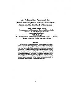
1.618     (8) h 1       1.283D84   In particular, Rickenmann and Recking (2011) reported that Eq. (7) performs the best in the

74

prediction of flow resistance, in comparison with other formulas including Eq. (8). Fig. 1

75

shows a comparison of Eqs. (3) to (8) by replacing r in Eq. (7) with h and plotting Eq. (4) with

76

St = 0.12. It can be seen that for 0.5 < h/D84 < 7, Eqs. (5) to (8) are close to each other, but

77

they differ from the two traditional formulas [Eqs. (3) and (4)].

1.904

 h  8  4.416   f  D84 

1.083

78

The present study aims to provide an alternative physical reasoning about flow

79

resistance induced by large-scale roughness. A resistance equation is thus developed, with

80

two coefficients to be calibrated with laboratory and field data available in the literature. 4

81 82 83

Theoretical consideration

84 85

The analysis presented in this section is based on the following assumptions: (1) The channel

86

is wide and the channel bed is planar and fully rough; (2) The flow is steady, turbulent, fully

87

developed and uniform; (3) The variation in the bed elevation is in the order of sediment

88

grain diameter D; and (4) The flow depth h is not large in comparison with D (e.g. 0 < h/D
.

1/ 2

177

To extend the above analysis to a mixed-size sediment bed, it is necessary to know

178

what sediment diameter should be selected to be a representative sediment size. Such a

179

selection is made generally by arguing that the representative size is greater than the

180

median diameter (Leopold et al. 1964). This is because grains of larger diameters protrude

181

above the average bed level and expose greater volume, and thus exert most of the

182

resistance to the flow (Whiting and Dietrich 1990). Perhaps for statistical reasons, the

183

representative diameter is often taken as D84 (for which 84% of sediment grains are finer), as 9

184

seen in various field data analyses (e.g. Bathurst 1985; Ferguson 2007; Hey 1979; Limerinos

185

1970; Rickenmann and Recking 2011; Whiting and Dietrich 1990). Therefore, in the following

186

analysis, D in Eq. (18) will be replaced with D84. In addition, h will be changed to the

187

hydraulic radius, r. In particular, by noting that laboratory experiments may be affected

188

significantly by sidewalls, a sidewall correction procedure will be applied to laboratory data,

189

which yields a corrected hydraulic radius, rb.

190 191 192

Calibrations

193 194

The two constants ( and ) in Eq. (18) can be evaluated using laboratory and field data. In

195

comparison with field studies, laboratory experiments are usually preformed under well-

196

controlled flow and bed conditions. First, Eq. (18) is fitted with laboratory data that meet the

197

requirements given in the foregoing derivation. As summarised in Table 1, in total 416 sets of

198

laboratory data were compiled from six sources, i.e. Paintal (1971), Bathurst et al. (1981), Ho

199

(1984), Cao (1985), Recking et al. (2008a) and Jordanova (2008). These data cover a range of

200

D84 (= 2.2-58 mm) and h/D84 (= 0.2-39.9). Bathurst et al. (1981) obtained their experimental

201

data for five different fixed roughness beds, each bed being one element thick. Paintal

202

(1971), Ho (1984), Cao (1985) and Recking et al. (2008a) have measured flow resistance with

203

and without bedload transport. The data of Paintal (1971), Cao (1985) and Recking et al.

204

(2008a) were tabulated in Recking (2006). The present analysis is limited to the datasets

205

with zero or negligible transport rate. Jordanova (2008) used hemispheres to simulate

206

roughness elements and measured flow resistance with different roughness densities for

207

submerged and emergent roughness conditions. Employed in this study is only part of 10

208

Jordanova’s data, which were measured under the condition of submerged, closely packed

209

hemispheres. In addition, D84 is taken as the diameter of hemispheres.

210

Of the 416 sets of data, 11% were collected under the narrow channel condition of

211

B/h < 5, where B is the channel width. To prepare the data for the calibration, the sidewall

212

correction was applied to all the laboratory data, which yields a corrected hydraulic radius rb

213

that is bed-related. The sidewall correction procedure employed here is the same as that

214

developed by Vanoni and Brooks (1957). With the cross-sectional average flow velocity V

215

and energy slope S, the friction factor f (= 8grS/V2) and Reynolds number R (= 4rV/) are first

216

calculated, where r [=Bh/(2h+B)] is the hydraulic radius and  is the kinematic viscosity of

217

fluid. Then the sidewall friction factor is evaluated using the relation, fw  31 ln1.3R / f 

218

(Cheng 2011b). Next, the bed friction factor is calculated with fb  2h  B  f  2hfw  / B .

219

Finally, the bed hydraulic radius is obtained as rb  rfb / f .

2.7

220

Plotted in Fig. 4 is the comparison of Eq. (18) with the data summarised in Table 1.

221

Three sets of - and -values are used for plotting Eq. (18), which describes the upper

222

bound of the data with  = 0 and  = 0.1, the lower bound with  = 0.1 and  = 0.3 and the

223

trend line with  = 0,  = 0.2. The trend line was obtained by comparing with the

224

experimental data of (8/f)1/2 with the results predicted using Eq. (18) for a series of  and 

225

combinations. The comparison shows that the average of the absolute error minimizes when

226

taking  = 0 and  = 0.2. Also shown in Fig. 4 are Manning-Strickler formula [Eq. (3) with St =

227

0.12], Keleugan formula [Eq. (4)] and Ferguson’s formula [Eq. (7)], the latter representing

228

field measurements. Fig. 4 shows that Manning-Strickler formula overestimates the value of

229

(8/f)1/2 for low submergence, the upper bound of the laboratory measurements of (8/f)1/2 is

230

close to Keulegan formula, and the lower bound is close to Ferguson’s formula. 11

231

Next, Eq. (18) is compared with field data (376 sets in total), which were compiled by

232

Ferguson (2007) from nine different sources. The same data was used by Ferguson (2007) for

233

fixing the two empirical coefficients in Eq. (7). Fig. 5 shows that the field data are generally

234

confined between the upper bound [Eq. (18) with  = 0 and  = 0.1] and the lower bound

235

[Eq. (18) with  = 0.4 and  = 0.6], and the trend line of the data can be described well by

236

Eq. (18) with  = 0.1 and  = 0.25. It can be also observed that the trend line agrees well

237

with Eq. (7), which is expected because of the same database used for calibration. It should

238

be mentioned that due to different choices of St, there is an offset between Ferguson’s

239

formula and Eq. (18) at the deep-flow side of the plot.

240

In addition, by comparing Figs. 4 and 5, it is noted that the trend line derived from

241

the laboratory data is slightly different from that from the field data. For a given r/D84, the

242

value of (8/f)1/2 observed in field is generally lower (and thus the resistance is larger) than

243

the laboratory measurement. In other words, for a given flow depth, the same friction factor

244

can be observed for both laboratory and field conditions provided that a greater roughness

245

element is employed in a laboratory experiment than in field. This is understandable by

246

noting bed surface irregularities that are usually higher in field than in a laboratory setup

247

even for a planar channel bed. With the two trend lines shown in Figs. 4 and 5, it can be

248

estimated that for a given flow depth, about 50% increase in D84 is needed in a laboratory

249

experiment to achieve the same friction factor as in field for r/D84 = 0.6-10.

250 251 252

Discussions

253 254

In the model derivation, the variation in the channel bed elevation is considered only with a 12

255

streamwise-vertical slice, as shown in Fig. 3. It should be noted that similar variations exist

256

also in the direction across the channel. For a shallow flow over such a ‘corrugated’ channel

257

bed, the water surface would not be planar, and the flow acceleration/deceleration would

258

be somewhat less than what has been calculated in the derivation. For example, if the bed

259

consists of an array of hemispherical stones, some lateral deflection of flow would occur

260

through the gaps between obstacles, which may result in less acceleration/deceleration over

261

their tops. Therefore, the head loss involved in the model derivation should be generally

262

replaced with a width-averaged head loss. This is worthy of further efforts in the future.

263

Eq. (18) fits well to both laboratory and field data. This can be attributed, in part, to

264

the use of the adjustable coefficients,  and . However, on the other hand, from the

265

derivation, it follows that both  and  are physically linked to geometrical properties of the

266

formed channel bed. For the regular bed surface, as sketched in Fig. 3, D measures the

267

average distance from the tops of obstacles to the mean bed level, while D quantifies the

268

average of the largest variations in the bed surface elevation. Therefore, for some two-

269

dimensional but regular bed configurations, it is possible to theoretically fix the two

270

coefficients based on the bed geometry. However, in the presence of irregular bed surfaces

271

as in real river beds, it may be necessary to apply a statistic or probabilistic approach to the

272

evaluation of the two coefficients. Recently, Coleman et al. (2011) reported that for water-

273

worked gravel beds, the crest-to-trough roughness height, hct, scales with the standard

274

deviation of bed elevations, b. They assumed that hct is equivalent to the median sediment

275

diameter and then obtained that hct = (1.8-2.4)b with b = 0.22D84. If taking hct = βD84, β can

276

be estimated to be 0.40-0.53. This range of β appears greater than β (= 0.2) used for the

277

laboratory data trend in Fig. 4 and β (= 0.25) for the field data trend in Fig. 5.

13

278

In addition,  and/or  may vary with the sediment size distribution. In the forgoing

279

calibration, D84 is used to be the representative sediment diameter. If D84 is replaced by a

280

diameter with another percentile, both  and  may have different values in the fitting of

281

Eq. (18) to the data. This implies that one or both of the two coefficients may also depend

282

on the sediment size distribution.

283

Finally, it should be mentioned that the proposed approach to the evaluation of

284

coarse-bed resistance applies only for the condition of planar rough beds. However, there

285

still exist other factors that may affect flow resistance significantly, particularly in natural

286

channels. For example, cross sections of natural stream channels can vary significantly in size

287

and shape, even within a short reach, which increases resistance to flows (Wohl 2010).

288

Further increases in flow resistance in natural coarse-bed streams occur in the presence of

289

pools and riffles (Maxwell and Papanicolaou 2001), boulders (Papanicolaou et al. 2012),

290

vegetation (Cheng 2011a; Darby and Thorne 1996), and large woody debris (Manga and

291

Kirchner 2000; Montgomery and Buffington 1997). Therefore, when fitting the coefficients α

292

and β to flow resistance measurements, the fitted values account for the additional effects

293

only in an average sense. This also explains why the large spreading of the data exists about

294

the “trend line”, particularly for values of r/D84 < 1. For example, Fig. 5 shows that the

295

measurement of 8 f at r/D84 = 0.3 varies from 0.03 to 2, a wide range in comparison to

296

0.75 calculated according to the proposed trend line.

297

Given the uncertainty in the prediction of resistance for large-scale roughness in

298

natural channels, the present approach may be further improved by taking into account the

299

other factors as mentioned above. For example, for a gravel bed subject to boulders, the bed

300

resistance may be partitioned into gravel-bed and boulder-affected components so that they

301

can be evaluated individually. Such an improvement could be made based on characteristics 14

302

of open channel flows over boulder-affected gravel beds, such as those presented by Thanos

303

Papanicolaou’s group in their recent studies (e.g. Hajimirzaie et al. 2014; Papanicolaou et al.

304

2011; Papanicolaou et al. 2012). Papanicolaou et al. (2012) investigated effects of a fully

305

submerged, wall-mounted boulder placed on a flat rough bed on mean and turbulent flow

306

fields. Their results show that the form roughness could be up to two times larger than the

307

skin roughness in the near-wake region of the boulder. Papanicolaou et al. (2012) also

308

reported that in comparison to a flat rough bed, the location of the maximum turbulence

309

intensity shifted away from the bed due to the vortices generated by the boulder. As a

310

result, the presence of boulder would enhance the vertical mixing near the bed and also

311

cause significant energy dissipation. For example, the average reach-averaged bed shear

312

stress increased by 30% when 40 isolated boulders were placed over a gravel bed, covering

313

only 2% of the bed area (Papanicolaou et al. 2011).

314 315 316

Summary

317 318

In this study, the rough bed surface is simplified as a periodic boundary to quantify energy

319

losses induced by the large scale roughness in open channel flows. The obtained analytical

320

resistance formula [Eq. (18)] is applicable for both deep and shallow flow conditions. It

321

reduces to the traditional Manning-Strickler formula when the flow depth is much greater

322

than the sediment size. The new formula was calibrated separately using laboratory and field

323

data. It is consistent with the best of previously-developed formulas in the prediction of flow

324

resistance for r/D84 = 0.1-10.

325 15

326 327

Acknowledgements

328

The author is grateful to the comments and additional references, provided by the reviewers

329

and editors.

330 331 332

Notation

333

The following symbols are used in this paper:

334

B

= channel width;

335

C

= Chezy coefficient;

336

D

= sediment grain diameter;

337

D84

= grain diameter of which 84% of the sediment is finer;

338

f

= Darcy-Weisbach friction factor;

339

fb

= bed friction factor;

340

fw

= sidewall friction factor;

341

g

= gravitational acceleration;

342

H

= nominal flow depth;

343

HC

= head loss due to contraction;

344

HE

= head loss due to expansion;

345

Hf

= head loss due to friction;

346

HL

= total head loss;

347

h

= average flow depth;

348

h1,h2,h3 = local flow depth;

349

hct

= crest-to-trough roughness height of sediment beds; 16

350

k

= representative roughness length;

351

L

= wave length;

352

n

= Manning coefficient;

353

q

= flow rate per unit width;

354

r

= hydraulic radius;

355

R

= 4rV/ = Reynolds number;

356

S

= energy slope;

357

St

= Strickler number or normalised Manning’s n;

358

U1,U2 = local depth-averaged velocity;

359

V

= cross-sectional average flow velocity;

360



= coefficient;

361



= coefficient;

362



= kinematic viscosity of fluid;

363



= h/D = relative flow depth; and

364

b

= standard deviation of the bed elevation.

365 366 367

References

368 369 370 371 372 373 374 375 376 377 378

Bathurst, J. C. (1978). " Flow resistance of large-scale roughness." Journal of the Hydraulics Division-ASCE, 104(12), 1587-1603. Bathurst, J. C. (1985). "Flow resistance estimation in mountain rivers." Journal of Hydraulic Engineering-ASCE, 111(4), 625-643. Bathurst, J. C., Li, R. M., and Simons, D. B. (1981). "Resistance equation for large-scale roughness." Journal of the Hydraulics Division-ASCE, 107(12), 1593-1613. Cao, H. H. (1985). "Resistance hydraulique d'un lit à gravier mobile à pente raide; étude expérimentale." Ph. D. Thesis, Ecole PolytechniqueFederale de Lausane. 17

379 380 381 382 383 384 385 386 387 388 389 390 391 392 393 394 395 396 397 398 399 400 401 402 403 404 405 406 407 408 409 410 411 412 413 414 415 416 417 418 419 420 421 422 423 424 425

Cheng, N. S. (2006). "Influence of shear stress fluctuation on bed particle mobility." Physics of Fluids, 18(9), 10.1063/1.2354434. Cheng, N. S. (2011a). "Representative roughness height of submerged vegetation." Water Resources Research, 47, 10.1029/2011wr010590. Cheng, N. S. (2011b). "Revisited Vanoni-Brooks sidewall correction." International Journal of Sediment Research, 26(4), 524-528. Chow, V. T. (1959). Open-channel hydraulics, McGraw-Hill, New York. Coleman, S. E., Nikora, V. I., and Aberle, J. (2011). "Interpretation of alluvial beds through bed-elevation distribution moments." Water Resources Research, 47, W11505, 10.1029/2011wr010672. Darby, S. E., and Thorne, C. R. (1996). "Predicting stage-discharge curves in channels with bank vegetation." Journal of Hydraulic Engineering-Asce, 122(10), 583-586, 10.1061/(asce)0733-9429(1996)122:10(583). Engelund, F., and Hansen, E. (1972). A monograph on sediment transport in alluvial streams, Technical Press, Copenhagen. Ferguson, R. (2007). "Flow resistance equations for gravel- and boulder-bed streams." Water Resources Research, 43(5), W05427, 10.1029/2006wr005422. Froehlich, D. C. (2012). "Resistance to Shallow Uniform Flow in Small, Riprap-Lined Drainage Channels." Journal of Irrigation and Drainage Engineering-ASCE, 138(2), 203-210, 10.1061/(asce)ir.1943-4774.0000383. Garcia, M. H. (2008). Sedimentation engineering: processes, measurements, modeling, and practice, American Society of Civil Engineers, Reston, Va. Goharzadeh, A., Khalili, A., and Jorgensen, B. B. (2005). "Transition layer thickness at a fluidporous interface." Physics of Fluids, 17(5), 10.1063/1.1894796. Hajimirzaie, S. M., Tsakiris, A. G., Buchholz, J. H. J., and Papanicolaou, A. N. (2014). "Flow characteristics around a wall-mounted spherical obstacle in a thin boundary layer." Experiments in Fluids, 55(6), 10.1007/s00348-014-1762-0. Hey, R. D. (1979). "Flow resistance in gravel-bed rivers." Journal of the Hydraulics DivisionASCE, 105(4), 365-379. Ho, C. M. (1984). "Study of bedload transport in turbulent open channel flows." Ph. D. Thesis, National Taiwan University, Taiwan. Jordanova, A. A. (2008). "Low flow hydraulics in rivers for environmental applications in 18

426 427 428 429 430 431 432 433 434 435 436 437 438 439 440 441 442 443 444 445 446 447 448 449 450 451 452 453 454 455 456 457 458 459 460 461 462 463 464 465 466 467 468 469 470 471 472

south Africa." Ph. D. Thesis, University of the Witwatersrand, Johannesburg. Katul, G., Wiberg, P., Albertson, J., and Hornberger, G. (2002). "A mixing layer theory for flow resistance in shallow streams." Water Resources Research, 38(11), 1250, 10.1029/2001wr000817. Keulegan, G. H. (1938). "Laws of turbulent flow in open channels." Journal of Research of the National Bureau of Standards, 21, 707-741. Lawrence, D. S. L. (2000). "Hydraulic resistance in overland flow during partial and marginal surface inundation: Experimental observations and modeling." Water Resources Research, 36(8), 2381-2393, 10.1029/2000wr900095. Leopold, L. B., Wolman, M. G., and Miller, J. P. (1964). Fluvial processes in geomorphology, W. H. Freeman & Co., San Francisco. Limerinos, J. T. (1970). Determination of the Manning coefficient from measured bed roughness in natural channels, United States Government Printing Office, Washington. Manes, C., Ridolfi, L., and Katul, G. (2012). "A phenomenological model to describe turbulent friction in permeable-wall flows." Geophysical Research Letters, 39, 10.1029/2012gl052369. Manga, M., and Kirchner, J. W. (2000). "Stress partitioning in streams by large woody debris." Water Resources Research, 36(8), 2373-2379, 10.1029/2000wr900153. Maxwell, A. R., and Papanicolaou, A. N. (2001). "Step-pool morphology in high-gradient streams." International Journal of Sediment Research, 16(3), 380-390. Montgomery, D. R., and Buffington, J. M. (1997). "Channel-reach morphology in mountain drainage basins." Geological Society of America Bulletin, 109(5), 596-611, 10.1130/00167606(1997)1092.3.co;2. Munson, B. R., Young, D. F., and Okiishi, T. H. (2006). Fundamentals of fluid mechanics, J. Wiley & Sons, Hoboken, NJ. Nikuradse, J. (1933). "Stromungsgesetze in rauhen Rohren." Forschung auf dem Gebiete des Ingenieurwesens, Forschungsheft 361. VDI Verlag, Berlin, Germany (in German). (English translation: Laws of flow in rough pipes, NACA TM 1292, 1950). Paintal, A. S. (1971). "Concept of critical shear stress in loose boundary open channels." Journal of Hydraulic Research, 9(1), 91-113. Papanicolaou, A. N., Dermisis, D. C., and Elhakeem, M. (2011). "Investigating the Role of Clasts on the Movement of Sand in Gravel Bed Rivers." Journal of Hydraulic EngineeringAsce, 137(9), 871-883, 10.1061/(asce)hy.1943-7900.0000381. Papanicolaou, A. N., Kramer, C. M., Tsakiris, A. G., Stoesser, T., Bomminayuni, S., and Chen, Z. 19

473 474 475 476 477 478 479 480 481 482 483 484 485 486 487 488 489 490 491 492 493 494 495 496 497 498 499 500 501 502 503 504 505 506 507 508 509

(2012). "Effects of a fully submerged boulder within a boulder array on the mean and turbulent flow fields: Implications to bedload transport." Acta Geophysica, 60(6), 1502-1546, 10.2478/s11600-012-0044-6. Recking, A. (2006). "An experimental study of grain Sorting effects on bedload." Ph. D. Thesis, University of Lyon, France. Recking, A., Frey, P., Paquier, A., Belleudy, P., and Champagne, J. Y. (2008a). "Bed-load transport flume experiments on steep slopes." Journal of Hydraulic Engineering-ASCE, 134(9), 1302-1310, 10.1061/(asce)0733-9429(2008)134:9(1302). Recking, A., Frey, P., Paquier, A., Belleudy, P., and Champagne, J. Y. (2008b). "Feedback between bed load transport and flow resistance in gravel and cobble bed rivers." Water Resources Research, 44(5), W05412 10.1029/2007wr006219. Rickenmann, D., and Recking, A. (2011). "Evaluation of flow resistance in gravel-bed rivers through a large field data set." Water Resources Research, 47, W07538, 10.1029/2010wr009793. Smart, G. M., Duncan, M. J., and Walsh, J. M. (2002). "Relatively rough flow resistance equations." Journal of Hydraulic Engineering-ASCE, 128(6), 568-578. Vanoni, V. A., and Brooks, N. H. (1957). "Laboratory studies of the roughness and suspended load of alluvial streams." Sedimentation Laboratory, California Institute of Technology, Pasadena, Calif. Whiting, P. J., and Dietrich, W. E. (1990). "Boundary shear stress and roughness over mobile aluvial beds." Journal of Hydraulic Engineering-ASCE, 116(12), 1495-1511. Wohl, E. (2010). Mountain rivers revisited, American Geophysical Union, Washington, DC. Yen, B. C. (1993). "Dimensionally homogeneous manning formula - closure." Journal of Hydraulic Engineering-ASCE, 119(12), 1443-1445, 10.1061/(asce)07339429(1993)119:12(1443).

510

20

Table Click here to download Table: Table 1.docx

Table 1. Summary of laboratory data used for calibration Investigator

Slope

Froude

Reynolds

D84

number

number

(mm)

1/2

Paintal (1970)

0.00117-

U/(gh)

4Uh/

0.43-0.98

7.410 -

0.02-0.08

dataset

2.9-24

4.0-39.9

34

11.5-58

0.3-6.1

88

2.2-15

1.1-35.9

168

14.3-54

0.8-10.1

50

2.4-9.6

1.2-34.7

64

47

0.2-2.6

12

9.910 0.19-1.93

3

4.410 5

(1981) Ho (1984)

Number of

5

0.0103 Bathurst et al.

4

h/D84

2.410 0.002-0.1

0.55-1.72

3

2.710 5

2.110 Cao (1985)

0.005-0.09

0.44-1.51

4

4.710 6

1.310 Recking (2008)

0.01-0.05

0.49-1.25

4

1.210 5

3.210 Jordanova

0.0011-

(2008)

0.0021

0.07-0.28

3

1.010 5

1.310

Figure1 Click here to download Figure: fig 1.pdf

10

8   f

1

Manning‐Strickler, Eq. (3) Keulegan, Eq. (4) Hey, Eq. (5) Katul et al., Eq. (6) Ferguson, Eq. (7) Rickenmann & Recking, Eq. (8)

0.1 0.1

1

      Fig. 1    Comparison of previous formulas   

 

 

10

h/D84 

100

 

Figure2 Click here to download Figure: fig 2.pdf

                     

h 

    Fig. 2    Open channel flow subject to large‐scale roughness (0