AN ALTERNATIVE NOTATION FOR REPRESENTING DENSE ...

AN ALTERNATIVE NOTATION FOR REPRESENTING DENSE LINEAR ALGEBRA ALGORITHMS ∗ PAOLO BIENTINESI∗ AND ROBERT A. VAN DE GEIJN∗ Abstract. We present a notation that allows a dense linear algebra algorithm to be represented in a way that is visually recognizable. The primary value of the notation is that it exposes subvectors and submatrices allowing the details of the algorithm to be the focus while hiding the intricate indices related to the arrays in which the vectors and matrices are stored. The applicability of the notation is illustrated through a succession of progressively complex case studies ranging from matrix-vector operations to the chasing of the bulge of the symmetric QR iteration. The notation facilitates comparing and contrasting different algorithms for the same operation as well as similar algorithms for different operations. Finally, we point out how algorithms represented with this notation can be directly translated into high-performance code. Key words. linear algebra, notation, algorithms, dense matrices, FLAME AMS subject classifications. 65F05, 65Y10.

1. Introduction. This paper showcases an alternative notation for representing, visually, algorithms for dense linear algebra operations. This notation has been effective for presenting well-known linear algebra algorithms in undergraduate and graduate courses and for presenting new algorithms in our recent papers [16, 18, 19, 27]. In addition, it has facilitated the systematic and automatic derivation of such algorithms [2, 4, 6, 14, 15, 26]. The strength of the notation is that it avoids indexing and that much of the high-level information that supports the algorithm is captured. Standard texts in numerical linear algebra, like those written by Golub and Van Loan [13], Demmel [7], Stewart [28], and many others, often develop the theory behind algorithms by partitioning matrices and then discussing how different submatrices are affected, updated, and/or used without the use of indices for exposing individual entries in matrices. By contrast, algorithms in these same texts are typically expressed by exposing intricate indices into the arrays that store matrices and vectors. The popularity of Matlab’s M-script language [25] for prototyping new algorithms supports and reinforces that view of how algorithms must be expressed: Algorithms are often presented in texts and other papers using “Matlab-like” notation. The disparity between how one reasons about algorithms and how they are then represented may have a number of possible roots. First, the area of numerical linear algebra developed at a time when typesetting papers and books was expensive. Because of this, it was important to represent algorithms concisely, in as little space as possible. We will see that representing algorithms with explicit indexing has this property. Second, the coding style for implementing the algorithms traditionally exposes explicit indexing. As a result, compilers were written to optimize code that exposed indexing. This then encouraged programmers to continue to write code in the same fashion, since compilers were reasonably good at optimizing such code. Papers and books have continued to present algorithms with exposed indices since it is perceived that this makes it easier for the reader to translate the algorithms to such traditional code. Finally, we have noticed that there are a number of people who reason about matrix algorithms in terms of indices. For them the traditional way of representing 1 Department of Computer Sciences, The University of Texas, Austin, TX 78712; phone: 512471-9720, fax: 512-471-8885, {pauldj,rvdg}@cs.utexas.edu. ∗ This work was supported in part by NSF grants ACR-0305163 and CCF-0342369.

1

2

P. BIENTINESI AND R. VAN DE GEIJN

algorithms is more natural. We will show that if concepts are naturally expressed via the partitioning of matrices (and/or vectors), and are often accompanied by pictures that focus on submatrices being updated and/or used, then algorithms can (and hould) similarly be expressed by tracking partitioned matrices (and/or vectors). Similarly, the statement of theorems and their proofs often involve the partitioning of matrices and vectors. It is these observation that naturally leads to a notation for expressing algorithms that deviates dramatically from the norm and from how algorithms are traditionally represented in code. The same observation should motivate how algorithms are to be coded, for example through Application Programming Interfaces (APIs) that mirror the notation used to express the algorithms [5]. The paper is organized as follows: Section 2 is a motivating example: first, it shows how algorithms for the Cholesky factorization are traditionally derived and represented; then, by contrast, the same algorithms are also displayed by means of a new representation. Sections 3, 4 and 5 are a parade of case studies to which the new notation is applied, starting from simple matrix-vector and matrix-matrix operations (Section 3), passing through the most common matrix factorizations (Section 4), and concluding with the more complicated QR algorithm (Section 5). Section 6 is a short discussion on a coding interface that closely mirrors the newly introduced notation, while Section 7 gives a final summary and comments. 2. A Motivating Example. In this section, the Cholesky factorization is used as a motivating example. We present a very quick review of what this operation entails, the theory that supports it, the classical derivation of one algorithm for computing it, how to attain high performance by casting the computation in terms of operations related to matrix-matrix multiplication, and finally our notation for expressing the algorithm. 2.1. The Cholesky factorization. This operation is only defined for symmetric positive definite matrices: Definition 2.1. A matrix A ∈ Rn×n is positive definite if and only if for all nonzero vectors x ∈ Rn it is the case that xT Ax > 0. We will prove the following theorem in Section 2.4: Theorem 2.2 (Cholesky Factorization Theorem). Given a symmetric positive definite (SPD) matrix A there exists a lower triangular matrix L such that A = LLT . The lower triangular matrix L is known as the Cholesky factor and LLT is known as the Cholesky factorization of A. It is unique if the diagonal elements of L are restricted to be positive. The operation that overwrites the lower triangular part of matrix A with its Cholesky factor will be denoted by A := Γ(A), which should be read as “A becomes its Cholesky factor.” Typically, only the lower (or upper) triangular part of A is stored, and it is that part that is then overwritten with the result. In this discussion, we will assume that the lower triangular part of A is stored and overwritten. 2.2. Application. The Cholesky factorization is used to solve the linear system Ax = y when A is SPD: Substituting the factors into the equation yields LLT x = y. Letting z = LT x, Ax = L (LT x) = Lz = y. | {z } z

3

REPRESENTING DENSE LINEAR ALGEBRA ALGORITHMS for j = 1 : n √ αj,j := αj,j

for j = 1 : n √ αj,j := αj,j 9 =

for i = j + 1 : n αi,j := αi,j /αj,j endfor

;

αj+1:n,j := αj+1:n,j /αj,j

9 > > > =

for k = j + 1 : n for i = k : n αi,k := αi,k − αi,j αk,j endfor endfor endfor

> > > ;

αj+1:n,j+1:n := αj+1:n,j+1:n − tril(αj+1:n,j αT j+1:n,j )

endfor

Fig. 2.1. Formulations of the Cholesky factorization that expose indices.

Thus, z can be computed by solving the triangular system of equations Lz = y and subsequently the desired solution x can be computed by solving the triangular linear system LT x = z. 2.3. Unblocked algorithm. The most common algorithm for computing A := Γ(A) can be derived as follows: Consider A = LLT . Partition µ ¶ µ ¶ α11 λ11 ? 0 (2.1) A= and L = . a21 A22 l21 L22 Remark 1. We adopt the commonly used notation where Greek lower case letters refer to scalars, lower case letters refer to (column) vectors, and upper case letters refer to matrices. The ? refers to a part of A that is neither stored nor updated. By substituting these partitioned matrices into A = LLT we find that µ

α11 a21

? A22

¶

µ =

λ11 l21

0 L22

¶µ

λ11 l21

0 L22

¶T

µ =

λ211 λ11 l21

? T + L22 LT22 l21 l21

¶ ,

from which we conclude that √ λ11 = α11 l21 = a21 /λ11

? . T L22 = Γ(A22 − l21 l21 )

These equalities motivate µ the algorithm ¶ α11 ? 1. Partition A → . a21 A22 √ 2. Overwrite α11 := λ11 = α11 . 3. Overwrite a21 := l21 = a21 /λ11 . T 4. Overwrite A22 := A22 − l21 l21 (updating only the lower triangular part of A22 ). 5. Continue with A = A22 . (Back to Step 1.) The algorithm is typically presented in a text using Matlab-like notation as illustrated in Fig. 2.1. Remark 2. Similar to the tril function in Matlab, we use tril(B) to denote the lower triangular part of matrix B.

4

P. BIENTINESI AND R. VAN DE GEIJN

2.4. Proof of the Cholesky Factorization Theorem. In this section, we partition A as in (2.1). The following lemmas, which can be found in any standard text, are key to the proof: Lemma 2.3. Let A ∈ Rn×n be SPD. Then α11 > 0. µ ¶ 1 Proof: Choose x = where 0 represents the vector of n − 1 zeroes. Then 0 µ ¶T µ ¶µ ¶ 1 α11 aT21 1 = α11 , 0 < xT Ax = 0 a21 A22 0 which proves the lemma. √ T Lemma 2.4. Let A ∈ Rn×n be SPD and l21 = a21 / α11 . Then A22 − l21 l21 is SPD. T Proof: Since A is symmetric so are A µ22 and ¶ A22 − l21 l21 . Let x1 6= 0 be an arbitrary χ0 vector of length n − 1. Define x = where χ0 = −xT1 a21 /α11 . Then, since x1 x 6= 0, ¶T µ ¶µ ¶ µ a21 aT21 χ0 α11 aT21 χ0 0 < xT Ax = = xT1 (A22 − )x1 x1 a21 A22 x1 α11 T = xT1 (A22 − l21 l21 )x1 . T is SPD. We conclude that A22 − l21 l21

Proof: [Cholesky Factorization Theorem] Proof by induction. Base case: n = 1 Clearly the result is true for a 1 × 1 matrix A = α11 : In this case, the fact that A is SPD means that α11 > 0 and its Cholesky factor is then given by √ λ11 = α11 . Inductive step: Assume the result is true for SPD matrix A ∈ R(n−1)×(n−1) . We will show that it holds for A ∈ Rn×n . Let A ∈ Rn×n be SPD. Partition A and L √ as in (2.1) and let λ11 = α11 (which is well-defined by Lemma 2.3), l21 = a21 /λ11 , T and L22 = Γ(A22 − l21 l21 ) (which exists thanks to Lemma 2.4 and the induction hypothesis). Then L is the desired Cholesky factor of A. By the principle of mathematical induction, the theorem holds. 2.5. Blocked algorithm. In order to attain high performance, the computation is cast in terms of matrix-matrix multiplication by so-called blocked algorithms. For the Cholesky factorization a blocked version of the algorithm can be derived by partitioning µ ¶ µ ¶ A11 ? L11 0 A→ and L → , A21 A22 L21 L22 where A11 and L11 are b×b. By substituting these partitioned matrices into A = LLT we find that ¶ µ ¶ µ ¶µ ¶T µ L11 LT11 ? ? 0 0 A11 L11 L11 . = = A21 A22 L21 L22 L21 L22 L21 LT11 L21 LT21 + L22 LT22 From this we conclude that L11 = Γ(A11 ) L21 = A21 L−T 11

? . L22 = Γ(A22 − L21 LT21 )

REPRESENTING DENSE LINEAR ALGEBRA ALGORITHMS

5

for j = 1 : n in steps of nb b := min(n − j + 1, nb ) Aj:j+b−1,j:j+b−1 := Γ(Aj:j+b−1,j:j+b−1 ) Aj+b:n,j:j+b−1 := Aj+b:n,j:j+b−1 A−T j:j+b−1,j:j+b−1 Aj+b:n,j+b:n := Aj+b:n,j+b:n − tril(Aj+b:n,j:j+b−1 AT j+b:n,j:j+b−1 ) endfor Fig. 2.2. Blocked algorithm for computing the Cholesky factorization. Here nb is the block size used by the algorithm.

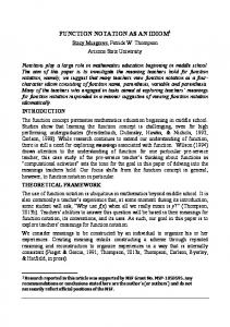
An algorithm is then described by the µ ¶ steps A11 ? 1. Partition A → , where A11 is b × b. A21 A22 2. Overwrite A11 := L11 = Γ(A11 ). 3. Overwrite A21 := L21 = A21 L−T 11 . 4. Overwrite A22 := A22 − L21 LT21 (updating only the lower triangular part). 5. Continue with A = A22 . (Back to Step 1.) An algorithm that explicitly indexes into the array that stores A is given in Fig. 2.2. Remark 3. The Cholesky factorization A11 := L11 = Γ(A11 ) can be computed with the unblocked algorithm or by calling the blocked Cholesky factorization algorithm recursively. Operations like L21 = A21 L−T 11 are computed by solving a linear system with multiple right-hand sides (TRSM). See also Section 3.2. 2.6. Alternative representation. When explaining the above algorithm in a classroom setting, invariably it is accompanied by a picture sequence like the one in Fig. 2.3(left) and the (verbal) explanation: Beginning of iteration: At some stage of the algorithm (Top of the loop), the computation has moved through the matrix to the point indicated by the thick lines. Notice that we have finished with the parts of the matrix that are in the top-left, top-right (which is not to be touched), and bottom-left quadrants. The bottom-right quadrant has been updated to the point where we only need to perform a Cholesky factorization of it. Repartition: We now repartition the bottom-right submatrix to expose α11 , a21 , and A22 . Update: α11 , a21 , and A22 are updated as discussed before. End of iteration: The thick lines are moved, since we now have completed more of the computation, and only a factorization of A22 (which becomes the new bottom-right quadrant) remains to be performed. Continue: The above steps are repeated until the submatrix ABR is empty. To motivate our notation, we annotate this progression of pictures as in Fig. 2.3 (right). In those pictures, “T”, “B”, “L”, and “R” stand for “Top”, “Bottom”, “Left”, and “Right”, respectively. This then motivates the format of the algorithm in Fig. 2.4 (left). A similar explanation can be given for the blocked algorithm, which is given in Fig. 2.4 (right). In the algorithms, m(A) indicates the number of rows of matrix A. Remark 4. The indices in our more stylized presentation of the algorithms are subscripts rather than indices in the conventional sense.

6

P. BIENTINESI AND R. VAN DE GEIJN done

done

done

partially updated

Beginning of iteration

AT L

?

ABL

ABR

↓

↓

Repartition

A00

?

?

aT 10

α11

?

A20

a21

A22

↓

↓

√ α11

UPD.

Update UPD.

↓ done

@ R @

done

A22 − a21 aT 21

a21 α11

UPD.

↓ done

AT L

?

ABL

ABR

End of iteration partially updated

Fig. 2.3. Left: Progression of pictures that explain Cholesky factorization algorithm. Right: Same pictures, annotated with labels and updates.

Remark 5. Clearly Fig. 2.4 does not present the algorithm as concisely as the algorithms given in Figs. 2.1 and 2.2. However, it does capture to a large degree the verbal description of the algorithm mentioned above and therefore, in our opinion, reduces both the effort required to interpret the algorithm and the need for additional explanations. The notation also mirrors that used for the proof in Section 2.4.

7

REPRESENTING DENSE LINEAR ALGEBRA ALGORITHMS

Algorithm: A := Chol unb(A) ţ ű AT L ? Partition A → ABL ABR where AT L is 0 × 0 while m(AT L ) < m(A) do

Algorithm: A := Chol blk(A) ţ ű AT L ? Partition A → ABL ABR where AT L is 0 × 0 while m(AT L ) < m(A) do Determine block size b Repartition 0 1 ţ ű A00 ? ? AT L ? → @ A10 A11 ? A ABL ABR A20 A21 A22 where A11 is b × b

Repartition 0 1 ţ ű A00 ? ? AT L ? → @ aT ? A 10 α11 ABL ABR A20 a21 A22 where α11 is 1 × 1 √ α11 := α11 a21 := a21 /α11 A22 := A22 − tril(a21 aT 21 )

A11 := Γ(A11 ) A21 := A21 tril(A11 )−T A22 := A22 − tril(A21 AT 21 )

Continue with 0 1 ţ ű ? A00 ? ? AT L T @ a10 α11 ? A ← ABL ABR A20 a21 A22 endwhile

Continue with 0 1 ţ ű ? A00 ? AT L ? @ A A A ? ← 10 11 ABL ABR A20 A21 A22 endwhile

Fig. 2.4. Unblocked and blocked algorithms for computing the Cholesky factorization.

Remark 6. The notation in Figs. 2.3 and 2.4 allows the contents of matrix A at the beginning of the iteration to be formally stated: ! µ ¶ Ã ? LT L AT L ? A= = , ABL ABR LBL AˆBR − tril(LBL LTBL ) ˆ ˆ ˆ where LT L = Γ(AˆT L ), LBL = AˆBL L−T T L , and AT L , ABL and ABR denote the original contents of the quadrants AT L , ABL and ABR , respectively. 3. Case Studies, Part I: Simple Operations. In this section, we discuss a cross-section of algorithms for simple linear algebra operations. These operations are among those supported by the widely used Basic Linear Algebra Subprograms (BLAS) [9, 8]. 3.1. Matrix-vector operations. Matrix vector operations are operations that take a matrix and one or more vectors as operands, and perform O(n2 ) operations when the matrix is n × n. Examples include different forms of matrix-vector multiplication (Matvec: y := αAx + βy), rank-1 update (Rank1: A := αxy + A), and the solution of a triangular system (Trsv: y := A−1 y, where A is a triangular matrix). We will focus on this last operation. Let U be an upper triangular matrix and consider the linear system U x = y. The Trsv operation overwrites y with the solution to this linear system, y := x = U −1 y. Partitioning µ U→

υ11 0

uT12 U22

¶

µ ,

x→

χ1 x2

¶

µ ,

and y →

η1 y2

¶ ,

8

P. BIENTINESI AND R. VAN DE GEIJN Algorithm: y := Trsv(U, y) Partition ţ ű ţ ű UT L UT R yT U → ,y→ 0 UBR yB where UBR is 0 × 0, yB has 0 elements while m(UBR ) < m(U ) do

Algorithm: Y := Trsm(U, Y ) Partition ţ ű ţ ű UT L UT R YT U → ,Y → 0 UBR YB where UBR is 0 × 0, YB has 0 rows while m(UBR ) < m(U ) do Determine block size b Repartition 0 1 ţ ű U00 U01 U02 UT L UT R @ 0 U U → 11 12 A, 0 UBR 0 0 U22 1 0 ţ ű Y0 YT → @ Y1 A YB Y2 where U11 is b × b, Y1 has b rows

Repartition 0 1 ţ ű U00 u01 U02 UT L UT R T @ 0 υ11 u12 A, → 0 UBR 0 0 U22 0 1 ţ ű y0 yT → @ η1 A yB y2 where υ11 and η1 are 1 × 1 Variant 1: η1 := η1 − uT 12 y2 η1 := η1 /υ11

Variant 1: Y1 := Y1 − U12 Y2 −1 Y1 := U11 Y1

Variant 2: η1 := η1 /υ11 y0 := y0 − u01 η1

Continue with 0 1 ţ ű U00 u01 U02 UT L UT R T ← @ 0 υ11 u12 A, 0 UBR 0 0 U22 0 1 ű ţ y0 yT ← @ η1 A yB y2 endwhile

Variant 2: −1 Y1 := U11 Y1 Y0 := Y0 − U01 Y1

Continue with 1 0 ţ ű U00 U01 U02 UT L UT R ← @ 0 U11 U12 A, 0 UBR 0 0 U22 0 1 ţ ű Y0 YT ← @ Y1 A YB Y2 endwhile

Fig. 3.1. Algorithms for the solution of a triangular system. Left: Single right-hand side. Right: −1 Multiple right-hand sides. We note that the operation Y1 := U11 Y1 is typically itself implemented as the computation of the solution of the smaller triangular system U11 X1 = Y1 , where X1 overwrites Y1 .

we have µ

υ11 0

uT12 U22

¶µ

χ1 x2

¶

µ =

η1 y2

¶

½ ,

or,

υ11 χ1 U22 x2

= η1 − uT12 x2 = y2 .

We conclude that if x2 has already been computed, overwriting y2 , then χ1 can be computed by χ1 = (η1 − uT12 y2 )/υ11 , overwriting η1 . The algorithm for this is given in Fig. 3.1(left), Variant 1. An alternative algorithm can be derived as follows: Partition µ ¶ µ ¶ µ ¶ U00 u01 x0 y0 U→ , x→ , and y → . 0 υ11 χ1 η1 Then

µ

U00 0

u01 υ11

¶µ

x0 χ1

¶

µ =

y0 η1

¶

½ ,

or,

U00 x0 + u01 χ1 υ11 χ1

= y0 = η1 ,

which suggests that χ1 can be computed by solving the second equation, overwriting η1 , after which y0 can be updated with y0 − η1 u01 . The computation continues by solving the smaller triangular system U00 x0 = y0 . These observations are represented in the algorithm in Fig. 3.1(left), Variant 2. As was mentioned for the Cholesky factorization in Remark 2.6, our notation allows us to mathematically describe the contents of vector y before and after execution

REPRESENTING DENSE LINEAR ALGEBRA ALGORITHMS

9

of the loop-iterations. Let yˆT and yˆB to respectively denote the original contents of yT and yB , then the algorithms for Variant 1 and 2 maintain in y the contents µ ¶ µ ¶ µ ¶ µ ¶ yT yˆT yT yˆT − UT R xB = and = , yB xB yB xB −1 respectively, where xB = UBR yˆB .

3.2. Matrix-matrix operations. Matrix-matrix operations are operations that take several matrices as operands and perform O(n3 ) operations on O(n2 ) data. Examples include different forms of matrix-matrix multiplication (Matmat: C := αAB + βC) and the solution of a triangular system with multiple right-hand sides (Trsm: Y := A−1 Y , where A is a triangular matrix). We will focus on this last operation as it is closely related to trsv. We will discuss algorithms that cast most computations in terms of matrix-matrix multiplications, for performance reasons [21]. Let U be an upper triangular matrix and consider the operation, Trsm, that overwrites Y := X under the constraint U X = Yˆ . Again, Yˆ denotes the original contents of matrix Y . Partition, conformally, µ ¶ µ ¶ µ ¶ µ ¶ UT L UT R XT YT YˆT ˆ U→ , X→ , Y → , and Y → . 0 UBR XB YB YˆB Then µ

UT L 0

UT R UBR

¶µ

XT XB

¶

µ =

YˆT YˆB

¶

½ ,

or,

UT L XT UBR XB

= YˆT − UT R XB = YˆB .

From this we conclude that XB should be computed before YˆT − UT R XB which in turn must be computed before XT . Two blocked algorithms for computing this operation are given in Fig. 3.1(right). Variant 1 and Variant 2 correspond to the algorithms that maintain in Y the contents µ ¶ µ ¶ µ ¶ µ ¶ YT YT YˆT YˆT − UT R XB = = and , YB YB XB XB −1 ˆ respectively, where XB = UBR YB .

Remark 7. In [2] we show how algorithms for this and other operations can be systematically derived. The new notation facilitates the methodology presented in that paper. 4. Case Studies, Part II: Factorization Algorithms. Next, we show how our notation can be used to represent algorithms for factoring matrices. In addition to a more thorough discussion of the Cholesky factorization, we review the LU factorization (with and without pivoting) and the QR factorization via Householder transformations. 4.1. Cholesky factorization, revisited. Let us define the computation of the ˆ where LLT = A, ˆ the Cholesky factorization as the overwriting of A := L = Γ(A) original contents of A. Partitioning the matrices we find that ¶µ ¶T µ 0 0 LT L LT L = LBL LBR LBL LBR

10

P. BIENTINESI AND R. VAN DE GEIJN

Algorithm: A := Chol unb(A) ű ţ AT L ? Partition A → ABL ABR where AT L is 0 × 0 while m(AT L ) < m(A) do Repartition 0 1 ţ ű A00 ? ? AT L ? → @ aT ? A 10 α11 ABL ABR A20 a21 A22 where α11 is 1 × 1

Algorithm: A := Chol blk(A) ű ţ AT L ? Partition A → ABL ABR where AT L is 0 × 0 while m(AT L ) < m(A) do Determine block size b Repartition 0 1 ţ ű A00 ? ? ? AT L → @ A10 A11 ? A ABL ABR A20 A21 A22 where A11 is b × b

Variant 1: T tril(A )−T aT 00 10 := a 10 q α11 := α11 − aT 10 a10

Variant 1:

Variant 2: q α11 := α11 − aT 10 a10 a21 := (a21 − A20 a10 )/α11

Variant 2:

Variant 3: √ α11 := α11 a21 := a21 /α11 A22 := A22 − tril(a21 aT 21 )

Variant 3: A11 := Γ(A11 ) A21 := A21 tril(A11 )−T A22 := A22 − tril(A21 AT 21 )

A10 := A10 tril(A00 )−T A11 := Γ(A11 − tril(A10 AT 10 )) A11 := Γ(A11 − tril(A10 AT 10 )) −T A21 := (A21 − A20 AT 10 ) tril(A11 )

Continue with 0 1 ű ţ A00 ? ? ? AT L T ← @ a10 α11 ? A ABL ABR A20 a21 A22 endwhile

Continue with 0 1 ţ ű A00 ? ? AT L AT R ← @ A10 A11 ? A ABL ABR A20 A21 A22 endwhile

Fig. 4.1. Unblocked and blocked algorithms for computing the Cholesky factorization.

µ =

LT L LTT L LBL LTT L

? LBL LTBL − LBR LTBR

Ã

¶ =

AˆT L AˆBL

? AˆBR

! ,

so that LT L = Γ(AˆT L ),

LBL = AˆBL L−T TL,

and

LBR = Γ(AˆBR − LBL LTBL ).

From this we note that LT L should be computed before LBL , which in turn should be computed before LBR : Upon completion of the factorization A must contain µ ¶ µ ¶ AT L ? LT L ? = . ABL ABR LBL LBR Previously, we saw that our notation allows us to identify algorithms by the contents that are maintained in the matrix or vector that is being updated. For the Cholesky factorization three possibilities are identified in Fig. 4.2. The algorithms (both unblocked and blocked) that maintain the indicated contents are given in Fig. 4.1. Remark 8. In [3] we show how algorithms for the Cholesky factorization can be systematically derived from the contents that are to be maintained in matrix by the algorithm.

11

REPRESENTING DENSE LINEAR ALGEBRA ALGORITHMS

µ

AT L ABL

Variant 1: ¶ µ LT L = ABR AˆBL ?

µ

AT L ABL

? ABR

Variant 2: ¶ µ LT L AT L ? = ABL ABR AˆBR LBL Variant 3: ¶ µ ¶ LT L ? = LBL AˆBR − tril(LBL LTBL ) ?

¶

µ

?

¶

AˆBR

Fig. 4.2. States maintained in matrix A corresponding to the algorithms given in Fig. 4.1 below.

4.2. LU factorization. Given a matrix A of size m × n with m ≥ n, its LU factorization is given by A = LU , where L is unit lower trapezoidal and U is upper triangular. This factorization is a reformulation of Gaussian Elimination and it exists ˆ to bring the atunder well-known conditions. We use the notation {L\U } = LU(A) tention to the fact that the function LU() takes a matrix A and returns two triangular matrices, L and U ; these two matrices can be stored overwriting the strictly lower and the upper triangular parts of A respectively. The diagonal of L consists of ones and is not stored. In the following discussion, {L\U }T L and {L\U }BR are abbreviations for {LT L \UT L } and {LBR \UBR }, respectively. Five unblocked algorithms have been proposed since Gauss first proposed Gaussian elimination. Partitioning the matrices into quadrants, we find that µ ¶µ ¶ µ ¶ LT L 0 UT L UT R LT L UT L LT L UT R = LBL LBR 0 UBR LBL UT L LBL UT R + LBR UBR à ! AˆT L AˆT R = , AˆBL AˆBR where Aˆ denotes the original contents of A. If A is to be overwritten with the final result, this means that upon completion A must contain µ ¶ µ ¶ AT L AT R {L\U }T L UT R = , ABL ABR LBL {L\U }BR where {L\U }T L = LU(AˆT L ) LBL = AˆBL UT−1 L

ˆ UT R = L−1 T L AT R . {L\U }T L = LU(AˆBR − LBL UT R )

In Fig. 4.3 we give five states maintained by the algorithms given in Fig. 4.4, which correspond to the five classic unblocked algorithms for computing the LU factorization [28], as well as their blocked counterparts. Remark 9. In [14] we show how algorithms for the LU factorization can be systematically derived from the contents that are to be maintained in matrix by the algorithm. 4.3. LU factorization with partial pivoting. It is well-known that the LU factorization is numerically unstable under general circumstances. In practice, LU factorization with partial pivoting solves these stability problems. For details on this subject we suggest the reader consult any standard text on numerical linear algebra.

12

P. BIENTINESI AND R. VAN DE GEIJN

ţ

ţ

AT L AT R ABL ABR AT L AT R ABL ABR

Variant à 1: ű

=

ˆT R {L\U }T L A ˆ ˆ ABL ABR

Variant à 3: ű

= ţ

ˆT R {L\U }T L A ˆ ABR LBL

AT L AT R ABL ABR

ű

!

!

ţ

ţ

AT L AT R ABL ABR AT L AT R ABL ABR

Variant à 2: ű

{L\U }T L UT R ˆBL ˆBR A A

=

Variant à 4: ű

{L\U }T L UT R ˆBR LBL A

=

!

!

ÃVariant 5: ! {L\U }T L UT R = ˆBR − LBL UT R LBL A

Fig. 4.3. States maintained in matrix A corresponding to the algorithms given in Fig. 4.4 below.

In this section, we will assume that the reader is familiar with the subject as we introduce new notation for presenting it. Definition 4.1. An n × n matrix P is said to be a permutation matrix, or T permutation, if, when applied to a vector x = (χ0 , χ1 , . . . , χn−1 ) , it merely rearranges the order of the elements in that vector. Such a permutation can be repreT sented by the vector of integers, (π0 , π1 , . . . , πn−1 ) , where {π0 , π1 , . . . , πn−1 } is a permutation of the integers {0, 1, . . . , n − 1} and the permuted vector P x is given by T (χπ0 , χπ1 , . . . , χπn−1 ) . If P is a permutation matrix then P A rearranges the rows of A exactly as the elements of x are rearranged by P x. We will see that when discussing the LU factorization with partial pivoting, a permutation matrix that swaps the first element of a vector with the π-th element of that vector is a fundamental tool. We will denote that matrix by         0 P (π) =  0      1    0

In 0 Iπ−1 0 0

if π = 0 

1 0  0 0   0 0 0 In−π−1

otherwise,

where n is the dimension of the permutation matrix. In the following we will use the notation Pn to indicate that the matrix P is of size n. Let p be a vector of integers satisfying the conditions T

(4.1)

p = (π0 , . . . , πk−1 ) , where 1 ≤ k ≤ n and 0 ≤ πi < n − i,

then Pn (p) will denote the permutation: µ Pn (p) =

Ik−1 0 0 Pn−k+1 (πk−1 )

¶µ

Ik−2 0 0 Pn−k+2 (πk−2 )

¶

µ ···

1 0 0 Pn−1 (π1 )

¶ Pn (π0 ).

Remark 10. In the algorithms, the subscript that indicates the matrix dimentions is omitted. Example 1. Let aT0 , aT1 , . . . , aTn−1 be the rows of a matrix A. The application of P (p) to A yields a matrix that results from swapping row aT0 with aTπ0 , then swapping aT1 with aTπ1 +1 , aT2 with aTπ2 +2 , until finally aTk−1 is swapped with aTπk−1 +k−1 .

REPRESENTING DENSE LINEAR ALGEBRA ALGORITHMS

Algorithm: A := LU unb(A) ţ ű AT L AT R Partition A → ABL ABR where AT L is 0 × 0 while n(AT L ) < n(A) do Repartition 1 0 ţ ű A00 a01 A02 AT L AT R T T → @ a10 α11 a12 A ABL ABR A20 a21 A22 where α11 is 1 × 1

Algorithm: A := LU blk(A) ţ ű AT L AT R Partition A → ABL ABR where AT L is 0 × 0 while n(AT L ) < n(A) do Determine block size b Repartition 1 0 ţ ű A00 A01 A02 AT L AT R → @ A10 A11 A12 A ABL ABR A20 A21 A22 where A11 is b × b

Variant 1: a01 := L−1 00 a01 T U −1 aT := a 10 10 00 α11 := α11 − aT 10 a01

Variant 1: A01 := L−1 00 A01 −1 A10 := A10 U00 A11 := LU(A11 − A10 A01 )

Variant 2: −1 T aT 10 := a10 U00 α11 := α11 − aT 10 a01 T T aT 12 := a12 − a10 A02

Variant 2: −1 A10 := A10 U00 A11 := LU(A11 − A10 A01 ) A12 := L−1 11 (A12 − A10 A02 )

Variant 3: a01 := L−1 00 a01 α11 := α11 − aT 10 a01 a21 := (a21 − A20 a01 )/α11

Variant 3: A01 := L−1 00 A01 A11 := LU(A11 − A10 A01 ) −1 A21 := (A21 − A20 A01 )U11

Variant 4: α11 := α11 − aT 10 a01 a21 := (a21 − A20 a01 )/α11 T T aT 12 := a12 − a10 A02

Variant 4: A11 := LU(A11 − A10 A01 ) −1 A21 := (A21 − A20 A01 )U11 −1 A12 := L11 (A12 − A10 A02 )

Variant 5: a21 := a21 /α11 A22 := A22 − a21 aT 12

Variant 5: A11 := LU(A11 ) −1 A21 := A21 U11 −1 A12 := L11 A12 A22 := A22 − A21 A12

Continue with 0 1 ţ ű A00 a01 A02 AT L AT R T A ← @ aT 10 α11 a12 ABL ABR A20 a21 A22 endwhile

13

Continue with 0 1 ţ ű A00 A01 A02 AT L AT R ← @ A10 A11 A12 A ABL ABR A20 A21 A22 endwhile

Fig. 4.4. Unblocked algorithm for computing the LU factorization. In this figure, n(A) is a function that yields the number of columns of matrix A and Lii and Uii denote the unit lower triangular matrix and upper triangular matrix stored over Aii , respectively.

Remark 11. For those familiar with how pivot information is stored in LINPACK and LAPACK, notice that those packages store the vector of pivot information T (π0 + 1, π1 + 2, . . . , πk−1 + k) .

14

P. BIENTINESI AND R. VAN DE GEIJN

Algorithm: [A, p] := LUpiv unb( A ) Partition ţ ű ţ ű AT L AT R pT A→ ,p→ ABL ABR pB where AT L is 0 × 0, pT has 0 elements while n(AT L ) < n(A) do Repartition 0 1 ţ ű A00 a01 A02 AT L AT R T A, → @ aT 10 α11 a12 ABL ABR A20 a21 A22 0 1 ű ţ p0 pT → @ π1 A pB p2 where α11 and π1 are scalars

Algorithm: [A, p] := LUpiv blk( A ) Partition ţ ű ţ ű AT L AT R pT A→ ,p→ ABL ABR pB where AT L is 0 × 0, pT has 0 elements while n(AT L ) < n(A) do Determine block size b Repartition 0 1 ţ ű A00 A01 A02 AT L AT R → @ A10 A11 A12 A, ABL ABR A20 A21 A22 0 1 ţ ű p0 pT → @ p1 A pB p2 where A11 is b × b , p1 is b × 1

Variant 3 (with pivoting):

Variant 3 (with pivoting):

a01 := L−1 00 a01 α11 := α11 − aT 10 a01 a A20 a01 21 := aű 21 − ÿ ůţ ţ ű α11 α11 , π1 := Pivot a21 a21 a21 := a21 /α11 ţ T ű ţ T ű aT aT a10 a10 12 12 := P (π1 ) A20 A22 A20 A22

A01 := L−1 00 A01 A11 := A11 − A10 A01 A21 := A21 − A20 A01 ÿ ţ ű ű ůţ A11 A11 , p1 := LUpiv A21 A21

Variant 4 (with pivoting):

Variant 4 (with pivoting):

ţ

aT 10 a01

α11 := α11 − a21 := a21 − A20 a01 T − aT A aT 02 12 := aű 12 ůţ ÿ 10 ţ ű α11 α11 , π1 := Pivot a21 a21 a21 := a21 /α11 ţ T ű ţ T a10 aT a10 12 := P (π1 ) A20 A22 A20 Variant 5 (with pivoting): ůţ ű ÿ ţ ű α11 α11 , π1 := Pivot a21 a21 a21 := a21 /α11 ţ T ű ţ T aT a10 a10 12 := P (π1 ) A20 A22 A20 A22 := A22 − a21 aT 12

aT 12 A22

aT 12 A22

ű

A10 A20

A12 A22

ű

ţ := P (p1 )

A10 A20

A12 A22

ű

A11 := A11 − A10 A01 A21 := A21 − A20 A01 A12 := A12 − A10 A02 ű ÿ ţ ű ůţ A11 A11 , p1 := LUpiv A21 A21 ţ ű ţ ű A10 A12 A10 A12 := P (p1 ) A20 A22 A20 A22 A12 := L−1 11 A12

ű

Continue with 0 1 ţ ű A00 a01 A02 AT L AT R T α T A @ a a ← , 11 10 12 ABL ABR A20 a21 A22 0 1 ţ ű p0 pT ← @ π1 A pB p2 endwhile

Variant 5 (with pivoting): ůţ ű ÿ ţ ű A11 A11 , p1 := LUpiv A21 A21 ţ ű ţ ű A10 A12 A10 A12 := P (p1 ) A20 A22 A20 A22 A12 := L−1 11 A12 A22 := A22 − A21 A12 Continue with 0 1 ţ ű A00 A01 A02 AT L AT R @ ← A10 A11 A12 A, ABL ABR A20 A21 A22 1 0 ţ ű p0 pT ← @ p1 A pB p2 endwhile

Fig. 4.5. Unblocked and blocked algorithms for LU factorization with partial pivoting. Here the matrix is pivoted like LAPACK does, so that P (p)A = LU upon completion. In this figure, Lii denotes the unit lower triangular matrix stored over Aii .

15

REPRESENTING DENSE LINEAR ALGEBRA ALGORITHMS

Having introduced our notation for permutation matrices, we can now define the LU factorization with partial pivoting: Given an m×n matrix A, with m ≥ n, we wish to compute a) a vector p of n integers which satisfies the conditions (4.1), b) a unit lower trapezoidal matrix L, and c) an upper triangular matrix U so that P (p)A = LU . An algorithm for computing this operation is typically represented by [A, p] := LUpiv(A), where upon completion A has been overwritten by {L\U }. Using our notation, unblocked and blocked algorithms for computing LUpiv are given in Fig. 4.5. Three variants are given, corresponding to the Variants 3–5 in Fig. 4.4 to which pivoting has been added. The function [x, π] = P ivot(x) determines the index of the element in vector x that has the maximal absolute value and swaps the first element of x with the maximal (in absolute value) element. 4.4. Computing an orthonormal basis. The goal of the Gram-Schmidt process is to compute an orthonormal basis for the space spanned by the columns of a given m × n matrix A (for m ≥ n) with n linearly independent columns. The vectors that constitute the orthonormal basis become the columns of an m × n matrix Q. A particular case of this problem can be stated as computing [Q, R] = QR(A), where R is an n × n upper triangular matrix so that A = QR. In this case, Q has the property that the first k columns of Q span the space spanned by the first k columns of A, for k = 1, . . . , n. Algorithms for computing Q and R can be described by partitioning A, Q, and R as ¶ µ ¡ ¢ ¡ ¢ RT L RT R A → AL AR , Q → QL QR , and R → , 0 RBR where AL and QL have k columns and RT L is k × k. Then ¶ µ ¡ ¢ ¡ ¢ RT L RT R AL AR = QL QR . 0 RBR Classical Gram-Schmidt. Assume that QL and RT L have already been computed. In other words, an orthonormal basis for AL has already been computed. Repartition, exposing columns to be updated, ¡ ¢ ¡ ¢ ¡ ¢ ¡ ¢ AL AR → A0 a1 A2 , QL QR → Q0 q1 Q2 , and µ

RT L 0

RT R RBR

¶



R00 → 0 0

r01 ρ11 0

 R02 T . r12 R22

Then  ¡

A0

a1

A2

¢

= =

¡ ¡

Q0

q1

Q0 R00

Q2

¢

R00  0 0

Q0 r01 + ρ11 q1

r01 ρ11 0

 R02 T  r12 R22

T Q0 R02 + q1 r12 + Q2 R22

¢

.

16

P. BIENTINESI AND R. VAN DE GEIJN

ą

CGS: AL AR

ć

=

ą

ˆR QL A

ć

ą

AL AR

ć

=

ą

MGS: ˆR − QL QT A ˆ QL A L R

ć

Fig. 4.6. States maintained in matrix A corresponding to the algorithms given in Fig. 4.7 below. Algorithm: [A, R] := QR(A) ţ ą ć RT L Partition A → AL AR ,R→ 0 where AL has 0 columns, RT L is 0 × 0 while n(AL ) < n(A) do Repartition ą

AL

AR

ć

→

ą

A0

a1

A2

ć

RT R RBR

ţ ,

RT L 0

ű

RT R RBR

0

ű

→@

R00 0 0

r01 ρ11 0

1 R02 T r12 A R22

where a1 has 1 column, ρ11 is a scalar MGS: ρ11 := ka1 k2 a1 := a1 /ρ11 T := aT A r12 1 2 T A2 := A2 − a1 r12

CGS: r01 := AT 0 a1 a1 := a1 − A0 r01 ρ11 := ka1 k2 a1 := a1 /ρ11 Continue with ć ą ą AL AR ← A0

a1

A2

ć

ţ ,

RT L RBL

RT R RBR

ű

0 ←@

R00 0 0

r01 ρ11 0

1 R02 T r12 A R22

endwhile Fig. 4.7. Orthogonalization via Gram-Schmidt and Modified Gram-Schmidt.

Now, Q0 and R00 have already been computed and we wish to compute the next column of Q and R. From a1 = Q0 r01 + ρ11 q1 , we deduce that QT0 a1 = r01 and q1 = (a1 − Q0 r01 )/ρ11 . Since q1 must have unit length, we find that the following steps compute q1 : Classical Gram-Schmidt (CGS) algorithm r01 := QT0 a1 q1 := a1 − Q0 r01 (= the component of a1 orthogonal to the columns of Q0 ) ρ11 := kq1 k2 q1 := q1 /ρ11 (normalization). This procedure is summarized in Fig. 4.7, where the process overwrites A with the orthogonal matrix Q. Modified Gram-Schmidt. The CGS algorithm is notoriously numerically unstable. More stable is the Modified Gram-Schmidt (MGS) algorithm. In this variant, every time a new column of Q, q1 , is computed, the remaining columns of A are updated by subtracting out the component of those columns that lies in the direction of q1 . Thus, at the beginning of a given step, a1 and A2 are already orthogonal to the columns of Q0 , which have overwritten A0 . The next column, q1 is then computed by normalizing the current contents of a1 . Finally, the columns of A2 are updated by subtracting out T T the component in the direction of q1 : A2 := A2 − q1 r12 , where r12 = q1T A2 . The MGS algorithm is also given in Fig. 4.7, and in Fig. 4.6 we show the states maintained in matrix A by the algorithms CGS and MGS.

REPRESENTING DENSE LINEAR ALGEBRA ALGORITHMS

17

4.5. QR factorization via Householder transformations. In this section, we introduce one unblocked algorithm for computing the QR factorization via Householder transformations. Enough background is given so that someone already familiar with this operation will be able to recognize how our notation supports it. Householder transformations. A Householder transformation (often called a reflector) is a matrix of the form H = I − βvv T , where v 6= 0 and β = 2/v T v. Notice that H = H T and H T H = H −1 H = I. In other words, H is orthogonal, symmetric, and equals its own inverse. µ ¶ µ ¶ χ1 χ1 ± kxk2 Now, let x 6= 0 and partition x → . If v is chosen as v = , x2 x2 ¶ µ ∓kxk2 holds. In other words, given a vector x, there exists then (I − βvv T )x = 0 a Householder transformation with the property that zeroes out the elements below the first element while preserving the norm of the vector1 . The ± is picked to equal the sign of χ1 , for numerical stability reasons. The discussion so far can be found in a typical numerical linear algebra text. We will now discuss how the vector that defines the Householder transformation can be chosen in a more practical way. Given the vector x, partitioned as before, we µ ¶ 1 1 T will define the Householder transformation instead as I − τ uu , where u = u2 and τ = uT u/2. Clearly this is simply a Householder transformation in disguise: The vector v in the Householder transformation can be scaled arbitrarily by scaling β correspondingly, and u is derived from v by dividing it by the first element of v. Thus, given a vector x, partitioned as before, u2 and τ now must satisfy à µ ¶µ ¶T ! µ ¶ µ ¶ 1 1 1 χ1 ρ I− = . u2 u2 x2 0 τ The following formulae compute u2 , τ , and ρ: ½ 0 if x = 0 u2 := x2 /(χ1 ± kxk2 ) otherwise τ := 2/uT u = 2/(1 + uT2 u2 ) ρ := ∓kxk2 . ¶ ¸ ρ , τ := h(x) as the function that computes We introduce the notation u2 the vector u2 , and scalars ρ and τ from the input vector x. Let A be an m × n with m ≥ n. We will now show how to compute the QR factorization A → QR , which, through a sequence of Householder transformations, eventually zeroes out all elements of matrix A below the diagonal. In the first iteration, we partition ¶ µ α11 aT12 . A→ a21 A22 ·µ

ţ 1 If

x = 0, then β is ill-defined. In that case, we will take v =

implementations take v = 0 and set β = 0.

1 0

ű and β = 2, although some

18

P. BIENTINESI AND R. VAN DE GEIJN Algorithm: [A, t] := QR(A) ţ ű ţ ű AT L AT R tT Partition A → ,s→ ABL ABR tB where AT L is 0 × 0, tT has 0 elements while n(ABR ) 6= 0 do Determine block size blank Repartition 0 ţ ű A00 a01 AT L AT R → @ aT α 11 10 ABL ABR A20 a21 where α11 and τ1 are scalars

1 0 1 ţ ű A02 t0 t T T → @ τ1 A a12 A, tB t2 A22

ůţ

ű ÿ ůţ ű ÿ ţ ű α11 η α11 , τ1 := , τ1 = h a21 u21 a21 T := (aT + uT A )/τ w12 22 1 12 21 T T aT 12 := a12 − w12 T A22 := A22 − u21 w12 Continue with 0 ţ ű A00 AT L AT R ← @ aT 10 ABL ABR A20 endwhile

a01 α11 a21

1 0 1 ţ ű A02 t0 t T T a12 A, ← @ τ1 A tB t2 A22

Fig. 4.8. Unblocked QR factorization algorithm.

Let ·µ

ρ11 u21

¶

¸ µ ¶ α11 , τ1 = h a21

be the Householder transform computed from the first column of A. Then applying this Householder transform to A yields à ¶ µ ¶µ ¶T ! µ ¶ µ 1 1 1 α11 aT12 α11 aT12 := I − a21 A22 u2 u2 a21 A22 τ µ ¶ T T ρ11 a12 − w12 = , T 0 A22 − u21 w12 T = (aT12 + uT21 A22 )/τ1 . Computation of a full QR factorization of A proceeds where w12 with the updated matrix A22 . The complete unblocked algorithm is given in Fig. 4.8.

Remark 12. We refer the interested reader to [16] for a more complete treatment of the QR factorization that presents unblocked and blocked algorithms as well as extensions that support out-of-core computation of a QR factorization. How to aggregate Householder transformations in support of a blocked algorithm is discussed in [18]. 5. Case Studies, Part III: The QR Algorithm. For the expert reader, we now discuss a much more advanced algorithm: The QR algorithm [11, 22], for computing the eigenvalues of a symmetric tridiagonal matrix T . We will assume that the reader is already intimately familiar with that algorithm. A good reference is [13]. For each iteration of this algorithm, the following steps are executed:

19

REPRESENTING DENSE LINEAR ALGEBRA ALGORITHMS

×× ××× ××× + ××× Beginning of iteration + ××× ××× ××× ×× ↓ ×× ××× ××× + ××× + ××× ××× ××× ×× ↓ ×× ××× ××× ××× + ××× + ××× ××× ×× ↓ ×× ××× ××× ××× + ××× + ××× ××× ××

TT L

T TM L

TM L

TM M

T TBM

TBM

TBR

↓ T00

t10

T T10

τ11

Repartition

tT 21

t21 T22

t32

tT 32

τ33

tT 43

t43 T44

↓

Update

T00

t10

tT 10

τ11

tT 21

t21 T22

t32

tT 32

τ33

tT 43

t43 T44

↓

End of iteration

TT L

T TM L

TM L

TM M

TBM

T TBM

TBR

Fig. 5.1. One step of “chasing the bulge” in the implicitly shifted symmetric QR algorithm.

• Determine a shift ρ (approximate eigenvalue of T ). • Determine a first Givens’ rotation G that annihilates the first element of the first subdiagonal of matrix T − ρI. • Update T := GT T G. This creates a nonzero in the first element of the second subdiagonal. • Determine Givens’ rotations that “chase the bulge” to make matrix t again tridiagonal. It is this last step that we discuss in this section.

20

P. BIENTINESI AND R. VAN DE GEIJN

Algorithm: T := ChaseBulge(T ) 0 1 TT L ? ? @ TM L TM M ? A Partition T → 0 TBM TBR where TT L is 0 × 0 and TM M is 3 × 3 while m(TBR ) > 0 do Repartition 0 T00 0 1 B tT TT L ? 0 B 10 @ TM L TM M ? A→B B 0 @ 0 0 TBM TBR 0 where τ11 and τ33 are scalars (during final step, τ33 is 0 × 0) ţ Compute (c, s) s.t. GT c,s t21 =

τ21 0

? τ11 t21 0 0

0 ? T22 tT 32 0

0 0 ? τ33 t43

1

0 0 0 ? T44

ű

ţ , and Assign t21 =

C C C C A

τ21 0

ű

T22 = GT c,s T22 Gc,s T tT 32 = t32 Gc,s

(not performed during final step)

Continue with 0 TT L ? @ TM L TM M 0 TBM

0

0 ? TBR

T00 B tT B 10 A←B 0 B @ 0 0 1

? τ11 t21 0 0

0 ? T22 tT 32 0

0 0 ? τ33 t43

0 0 0 ? T44

1 C C C C A

endwhile Fig. 5.2. Chasing the bulge.

A typical intermediate stage in the chasing of the bulge is illustrated in Fig. 5.1. We are now using more lines to track progress through the matrix: An initial 3 × 3 partitioning becomes a 5×5 partitioning, which then becomes again a 3×3 partitioning to set up the next iteration. This example gives us the opportunity to ask the question why in the other examples matrices were partitioned into a 2 × 2 partitioning and repartitioned to a 3 × 3 partitioning. The answer is that a 2 × 2 partitioning is needed to track the four quadrants. To be able to identify the submatrices that are moved from one side of the thick line to the other, the two 2 × 2 partitionings are superimposed, creating the familiar 3 × 3 partitioning. In order to identify the bulge, a 3 × 3 partitioning is needed at the top of the loop, as well as at the bottom of the loop, as illustrated in the left-most and rightmost pictures in Fig. 5.1. By superimposing these two pictures, the 5 × 5 partitioning appears, which now identifies submatrices that are to be moved across the thick line boundaries. The resulting algorithm for chasing the bulge is now given in Fig. 5.2. 6. Representing Algorithms in Code. The notation we presented does not closely resemble how algorithms have traditionally been represented in code. In this section we show that it is possible to easily define an API for a target language that allows the code to closely mirror the algorithm. The translation of the algorithm to traditional Matlab code still introduces a complicated indexing, as is shown in Fig. 6.1 for the blocked algorithm of Fig. 2.4. In order to overcome the indexing, we suggest coding algorithms in the style illustrated

REPRESENTING DENSE LINEAR ALGEBRA ALGORITHMS

n = size(A,1); for j=1:nb:n b = min( n-j+1, nb A(j:j+b-1,j:j+b-1) A(j+b:n,j:j+b-1) A(j+b:n,j+b:n)

21

); = Chol(A(j:j+b-1,j:j+b-1)); = A(j+b:n,j:j+b-1) / tril( A(j:j+b-1,j:j+b-1); = A(j+b:n,j+b:n) - ... tril(A(j+b:n,j:j+b-1)*A(j+b:n,j+b-1)’);

end Fig. 6.1. Traditional Matlab code for blocked Cholesky factorization (Variant 3).

function [ A_out ] = Chol_blk( A, nb_alg ) [ ATL, ATR, ... ABL, ABR ] = FLA_Part_2x2( A, ... 0, 0, ’FLA_TL’ ); while ( size( ATL, 1 ) < size( A, 1 ) ) b = min( size( ABR, 1 ), nb_alg ); [ A00, A01, A02, ... A10, A11, A12, ... A20, A21, A22 ] = FLA_Repart_2x2_to_3x3( ATL, ATR, ... ABL, ABR, ... b, b, ’FLA_BR’ ); %------------------------------------------------------------% A11 = Chol_unb( A11 ); A21 = A21 / tril( A11 )’; A22 = A22 - tril( A21 * A21’ ); %------------------------------------------------------------% [ ATL, ATR, ... ABL, ABR ] = FLA_Cont_with_3x3_to_2x2( A00, A01, A02, ... A10, A11, A12, ... A20, A21, A22, ... ’FLA_TL’ ); end A_out = [ ATL, ATR ABL, ABR ]; return

Fig. 6.2. FLAME@lab (Matlab) code for a blocked Cholesky factorization (Variant 3).

in Fig. 6.2. For details on this API and similar APIs for other programming languages, we refer the reader to [5]. The Linear Algebra Package (LAPACK) [1] is a widely used package that supports a broad set of dense linear algebra operations. It casts most computation in terms of calls to the Basic Linear Algebra Subprograms (BLAS) [24, 9, 8]. A code segment from the LAPACK routine for the blocked LU factorization with pivoting is given in Fig. 6.3. Clearly, there is the opportunity for the introduction of indexing errors. Indeed, we challenge the reader to find the errors that we purposely introduced. In Fig. 6.4 we show an implementation of the same algorithm using the FLAME/C API [14]. We believe that our API naturally captures the algorithm as presented using our notation, thereby reducing the opportunity for the introduction of inadvertent coding errors. A similar API for FORTRAN has also been defined. The translation

22

P. BIENTINESI AND R. VAN DE GEIJN

DO 20 J = 1, MIN( M, N ), NB JB = MIN( MIN( M, N )-J+1, NB ) * * * *

Factor diagonal and subdiagonal blocks and test for exact singularity. CALL DGETF2( M-J+1, JB, A( J, J ), LDA, IPIV( J ), IINFO )

* * *

Adjust INFO and the pivot indices.

$

10 * * *

IF( INFO.EQ.0 .AND. IINFO.GT.0 ) INFO = IINFO + J - 1 DO 10 I = J, MIN( M, J+JB+1 ) IPIV( I ) = J - 1 + IPIV( I ) CONTINUE Apply interchanges to columns 1:J-1. CALL DLASWP( J-1, A, LDA, J, J+JB+1, IPIV, 1 )

* IF( J+JB.LE.N ) THEN * * *

Apply interchanges to columns J+JB:N. CALL DLASWP( N-J-JB-1, A( 1, J+JB ), LDA, J, J+JB+1, IPIV, 1 )

* * *

Compute block row of U.

$ * * *

CALL DTRSM( ’Left’, ’Lower’, ’No transpose’, ’Unit’, JB, N-J-JB-1, ONE, A( J, J ), LDA, A( J, J+JB ), LDA ) IF( J+JB.LE.M ) THEN Update trailing submatrix.

$ $

20

CALL DGEMM( ’No transpose’, ’No transpose’, M-J-JB-1, N-J-JB-1, JB, -ONE, A( J+JB, J ), LDA, A( J, J+JB ), LDA, ONE, A( J+JB, J+JB ), LDA ) END IF END IF CONTINUE

Fig. 6.3. LAPACK code for blocked LU factorization (Variant 5 with pivoting).

of algorithm to code is essentially equivalent to the application of simple rewrite rules to that algorithm. Indeed, an API has been defined even for G, the graphical programming language that underlies LabView [20]. One word on performance: For blocked algorithms the additional cost of hiding intricate indices in code via the appropriate APIs is amortized over enough computation that it does not adversely affect performance. Often times the overhead is instead noticeable for unblocked algorithms. However, the code as presented in Figures 6.2 and 6.4 passes to a compiler a lot more high-level information than does code that exposes intricate indices. Compilers like those pursued by the Broadway project [17] could enable the generation of highly optimized implementations from algorithms expressed at this level of abstraction. A recent topic of research relates to the storage of matrices by blocks rather than the traditional row- or column-major orderings [10, 12, 29]. Our notation and the new

REPRESENTING DENSE LINEAR ALGEBRA ALGORITHMS

23

while (b = min(min(FLA_Obj_length( ABR ), FLA_Obj_width( ABR )), nb_alg) ) { FLA_Repart_2x1_to_3x1( ipivT, &ipiv0, /* ***** */ /* ***** */ &ipiv1, ipivB, &ipiv2, b, /* length ipiv1 split from */ FLA_BOTTOM ); FLA_Repart_2x2_to_3x3( ATL, /**/ ATR, &A00, /**/ &A01, &A02, /* ************* */ /* ********************* */ /**/ &A10, /**/ &A11, &A12, ABL, /**/ ABR, &A20, /**/ &A21, &A22, b, /* by */ b, /* A11 split from */ FLA_BR ); /* ********************************************************************* */ FLA_LU_unb( A11, A21, ipiv1 ); FLA_Apply_pivots( FLA_LEFT, FLA_NO_TRANSPOSE, ipiv1, A10, A20 ); FLA_Apply_pivots( FLA_LEFT, FLA_NO_TRANSPOSE, ipiv1, A12, A22 ); FLA_Trsm( FLA_LEFT, FLA_LOWER_TRIANGULAR, FLA_NO_TRANSPOSE, FLA_UNIT_DIAG, ONE, A11, A12 ); FLA_Gemm( FLA_NO_TRANSPOSE, FLA_NO_TRANSPOSE, MINUS_ONE, A21, A12, ONE, A22 ); /* ********************************************************************* */ FLA_Cont_with_3x3_to_2x2( &ATL, /**/ &ATR, A00, A01, /**/ A02, /**/ A10, A11, /**/ A12, /* ************** */ /* ****************** */ &ABL, /**/ &ABR, A20, A21, /**/ A22, /* with A11 added to submatrix */ FLA_TL ); FLA_Cont_with_3x1_to_2x1( &ipivT,

ipiv0, ipiv1, /* ***** */ /* ***** */ &ipivB, ipiv2, /* with ipiv1 added to */ FLA_TOP );

}

Fig. 6.4. FLAME code for blocked LU factorization (Variant 5 with pivoting).

APIs allow the very complex indexing associated with such storage to be completely hidden from the programmer. An alternative (and in our view better) solution to this problem is to allow matrices to have entries that themselves are matrices, which can also be accommodated by our notation and APIs [5]. 7. Conclusion. The contribution of the presented notation is that it allows algorithms to be expressed at the level of abstraction of the underlying theory. Our notation embraces the notion of subvectors and submatrices while hiding the physical arrays that store them. The manner in which compution sweeps through vectors and matrices is often consistent across different algorithms for computing the same operation. It is how subvectors and aubmatrices are updated that differs. This important insight is typically obscured by algorithms that explicitly expose indices. Conversely, our notation

24

P. BIENTINESI AND R. VAN DE GEIJN

highlights this commonality, and thus allows different algorithmic variants to be easily compared and contrasted. Likewise commonalities and differences between algorithms for different operations can be exhibited. The presentation of multiple variants for the same operation leads to some obvious questions. How can one find all loop-based algorithmic variants for a given linear algebra operation? Are there more variants than we have presented? Are all variants numerically stable? What are the performance benefits of one variant over another? What is the relationship between loop-based algorithms and recursive algorithms? Indices add a level of complexity to the problem that obscures the mathematical statement of these questions and makes it harder to answer them. Our recent research presents evidence that the proposed notation facilitates the formal statement of these questions as well as their answers. In [2] we present a systematic approach for deriving loop-based algorithms. We show the methodology to be sufficiently systematic to enable mechanical (automatic) generation of algorithms in [4], while initial results regarding numerical stability are given in [6]. A comparative study of the performance benefits for a family of algorithms is provided in [3]. A final comment on the typesetting of algorithms: we have developed a set of simple commands for typing algorithms using our notation in LATEX [23]. These commands have been used by undergraduate and graduate students with no previous exposure to LATEX in classes that we have taught. More information. Visit http://www.cs.utexas.edu/users/flame/. Acknowledgments. We would like to thank Peter Brune, Margaret Myers, Monika Petera, Enrique Quintana-Ort´ı, Field Van Zee, and Petko Yanev for their comments on drafts of this paper. REFERENCES [1] E. Anderson, Z. Bai, C. Bischof, L. S. Blackford, J. Demmel, J. J. Dongarra, J. D. Croz, S. Hammarling, A. Greenbaum, A. McKenney, and D. Sorensen, LAPACK Users’ guide (third ed.), Society for Industrial and Applied Mathematics, Philadelphia, PA, USA, 1999. [2] P. Bientinesi, J. A. Gunnels, M. E. Myers, E. S. Quintana-Ort´ı, and R. A. van de Geijn, The science of deriving dense linear algebra algorithms, ACM Trans. Math. Soft., 31 (2005), pp. 1–26. [3] P. Bientinesi, B. Gunter, and R. van de Geijn, High performace and parallel inversion of a symmetric positive definite matrix, SIAM J. Sci. Comput. submitted. [4] P. Bientinesi, S. Kolos, and R. van de Geijn, Automatic derivation of linear algebra algorithms with application to control theory, in Proceedings of PARA’04 State-of-the-Art in Scientific Computing, June 20-23 2004. To appear. [5] P. Bientinesi, E. S. Quintana-Ort´ı, and R. A. van de Geijn, Representing linear algebra algorithms in code: The FLAME APIs, ACM Trans. Math. Soft., 31 (2005), pp. 27–59. [6] P. Bientinesi and R. van de Geijn, Formal correctness and stability of dense linear algebra algorithms, in Proceedings of the 17th IMACS World Congress: Scientific Computation, Applied Mathematics and Simulation, July 11-16 2005. To appear. [7] J. W. Demmel, Applied numerical linear algebra, Society for Industrial and Applied Mathematics, Philadelphia, PA, USA, 1997. [8] J. J. Dongarra, J. Du Croz, S. Hammarling, and I. Duff, A set of level 3 basic linear algebra subprograms, ACM Trans. Math. Soft., 16 (1990), pp. 1–17. [9] J. J. Dongarra, J. Du Croz, S. Hammarling, and R. J. Hanson, An extended set of FORTRAN basic linear algebra subprograms, ACM Trans. Math. Soft., 14 (1988), pp. 1–17. ¨ m, Recursive blocked algorithms [10] E. Elmroth, F. Gustavson, I. Jonsson, and B. K˚ agstro and hybrid data structures for dense matrix library software, SIAM Review, 46 (2004), pp. 3–45.

REPRESENTING DENSE LINEAR ALGEBRA ALGORITHMS

25

[11] G. J. F. Francis, The QR transformation, parts I and II, Computer J., 4 (1961-62), pp. 265– 271,332–345. [12] J. D. Frens and D. S. Wise, Auto-blocking matrix-multiplication or tracking blas3 performance with source code, in PPoPP97, June 1997. [13] G. H. Golub and C. F. Van Loan, Matrix Computations, The Johns Hopkins University Press, Baltimore, 3nd ed., 1996. [14] J. A. Gunnels, F. G. Gustavson, G. M. Henry, and R. A. van de Geijn, FLAME: Formal linear algebra methods environment, ACM Transactions on Mathematical Software, 27 (2001), pp. 422–455. [15] J. A. Gunnels and R. A. van de Geijn, Formal methods for high-performance linear algebra libraries, in The Architecture of Scientific Software, R. F. Boisvert and P. T. P. Tang, eds., Kluwer Academic Press, 2001, pp. 193–210. [16] B. Gunter and R. van de Geijn, Parallel out-of-core computation and updating of the QR factorization, ACM Trans. Math. Soft., (2005). [17] S. Z. Guyer and C. Lin, Broadway: A Software Architecture for Scientific Computing, Kluwer Academic Press, October 2000, pp. 175–192. [18] T. Joffrain, T. M. Low, E. S. Quintana-Ort´ı, R. van de Geijn, and F. V. Zee, On accumulating Householder transformations, TOMS. in revision. [19] T. Joffrain, E. S. Quintana-Ort´ı, and R. A. van de Geijn, Rapid development of highperformance out-of-core solvers for electromagnetics, in Proceedings of PARA’04 State-ofthe-Art in Scientific Computing, June 20-23 2004. To appear. [20] G. W. Johnson, R. Jennings, and R. Jennigns, LabVIEW Graphical Programming, McGrawHill. ¨ m, P. Ling, and C. V. Loan, GEMM-based level 3 BLAS: High performance [21] B. K˚ agstro model implementations and performance evaluation benchmark, ACM Trans. Math. Soft., 24 (1998), pp. 268–302. [22] V. N. Kublanovskaya, On some algorithms for the solution of the complete eigenvalue problem, Zh. Vych. Mat., 1 (1961), pp. 555–570. [23] L. Lamport, LATEX: A Document Preparation System, Addison-Wesley, Reading, MA, 1986. [24] C. L. Lawson, R. J. Hanson, D. R. Kincaid, and F. T. Krogh, Basic linear algebra subprograms for Fortran usage, ACM Trans. Math. Soft., 5 (1979), pp. 308–323. [25] C. Moler, J. Little, and S. Bangert, Pro-Matlab, User’s Guide, The Mathworks, Inc., 1987. [26] E. S. Quintana-Ort´ı and R. A. van de Geijn, Formal derivation of algorithms: The triangular Sylvester equation, ACM Transactions on Mathematical Software, 29 (2003), pp. 218– 243. [27] G. Quintana-Ort´ı and R. van de Geijn, Improving the performance of reduction to Hessenberg form, ACM Trans. Math. Soft. Accepted for publication. [28] G. W. Stewart, Introduction to Matrix Computations, Academic Press, Orlando, Florida, 1973. [29] V. Valsalam and A. Skjellum, A framework for high-performance matrix multiplication based on hierarchical abstractions, algorithms and optimized low-level kernels. Concurrency and Computation: Practice and Experience, 2002.