This approach was originally identified in a case-based spam filtering ...... nation. In K. D. Ashley and D. G. Bridge, editors, Case-Based Reasoning Research ...
B LAME -BASED N OISE R EDUCTION : A N A LTERNATIVE P ERSPECTIVE ON N OISE R EDUCTION FOR L AZY L EARNING
Blame-Based Noise Reduction: An Alternative Perspective on Noise Reduction for Lazy Learning∗ François-Xavier Pasquier
FRANCOIS . XAVIER @ M 4 TP. ORG
Computer Science Department Trinity College Dublin Dublin 2, Ireland
Sarah-Jane Delany
SARAHJANE . DELANY @ COMP. DIT. IE
School of Computing Dublin Institute of Technology Kevin St., Dublin 8, Ireland
Pádraig Cunningham
PADRAIG . CUNNINGHAM @ CS . TCD . IE
Computer Science Department Trinity College Dublin Dublin 2, Ireland
Editor:
Abstract In this paper we present a new perspective on noise reduction for nearest-neighbour classifiers. Classic noise reduction algorithms such as Repeated Edited Nearest Neighbour remove cases from the training set if they are misclassified by their nearest neighbours in a leave-one-out cross validation. In the approach presented here, cases are identified for deletion based on their propensity to cause misclassifications. This approach was originally identified in a case-based spam filtering application where it became clear that certain training examples were damaging to the accuracy of the system. In this paper we evaluate the general applicability of the approach on a large variety of datasets and show that it generally beats the classic approach. We also compare the two techniques on artificial noise and show that both are far from perfect at removing noise and that there remains scope for further research in this area. Keywords: Nearest-Neighbour Classifiers, Noise Reduction.
0. This research was supported by funding from Enterprise Ireland under grant no. CFTD/03/219 and funding from Science Foundation Ireland under grant no. SFI-02IN.1I111
1
PASQUIER , D ELANY AND C UNNINGHAM
1. Introduction Because nearest neighbour classifiers (case-based classifiers) are local learners they can be very susceptible to noise. This can be overcome to a great extent by using more than one neighbour (k > 1) in classification. Nevertheless, there is still a great deal of interest in removing noisy training examples in case-based classifiers (Wilson, 1972; Tomek, 1976). There has been a resurgence of interest in recent years because noise reduction is a key issue in case-base editing (McKenna and Smyth, 2000; Wilson and Martinez, 1997; Brighton and Mellish, 2002). Noise reduction is useful not only to improve the accuracy of a case-based classifier but also in situations where cases will be retrieved for use in explanation (Roth-Berghofer (2004)) as inaccurate cases will undermine the credibility of the explanation. In this paper we present a novel approach which we call Blame-Based Noise Reduction (BBNR) for identifying noisy cases that are candidates for deletion. This approach was developed while optimising the performance of a case-based spam filtering system (Delany and Cunningham, 2004). In the spam filtering work, it was possible to home in on the cause of misclassifications and it became clear that certain training cases were unhelpful and would be better removed. In some situations these cases were genuinely noise (i.e. mislabeled). In other situations they were not noise in the true sense but nevertheless caused misclassifications; for instance this occurred with spam training examples that looked like legitimate email. Such cases were indistinguishable from legitimate email in the representation on which the classifier worked. This insight suggested that a deletion policy based on an analysis of the damage done by training cases could be effective. This contrasts with traditional noise reduction mechanisms which tend to focus on removing the actual cases that are misclassified. The dominant technique in this area is Repeated Edited Nearest Neighbour (RENN) (Tomek, 1976). Our earlier work shows that our noise deletion policy (BBNR) improved the accuracy of our spam filtering system and was more effective than RENN (Delany and Cunningham, 2004). The evaluation we present here shows that this generally holds true for other datasets, however the improvements in accuracy from both techniques are often disappointing. The noise reduction technique we present extends the competence-based modelling ideas of Smyth and colleagues (Smyth and Keane, 1995; Smyth and McKenna, 1998). Their case coverage measure indicates how well a case contributes to correctly classifying other cases in the case-base. We extend this model to include the notion of blame or liability. We introduce a measure of how often a case contributes to the misclassification of other cases. This information is gathered as part of an off-line leave-one-out analysis of the training data. BBNR as outlined is a principle on which a family of noise deletion policies can be based. Two such policies are presented in section 2. The traditional RENN approach is also described in section 2. In section 3 both approaches are evaluated on 20 datasets and in section 4 the techniques are evaluated on data with varying levels of artificial noise in an attempt to gain some insight into the relative strengths of the two techniques. The paper concludes in section 5 with some suggestions for future work.
2. Nearest Neighbour Classifiers and Noise Reduction This section discusses how noise reduction fits into the more general area of case-base editing and outlines the existing noise reduction techniques. It discusses BBNR, our new approach to noise 2
B LAME -BASED N OISE R EDUCTION : A N A LTERNATIVE P ERSPECTIVE ON N OISE R EDUCTION FOR L AZY L EARNING
reduction and describes the extensions to the models of case-base competence on which BBNR is based. It also defines two possible deletion policies for BBNR. 2.1 Noise Reduction in Case-Base Editing There has been significant work on case-base editing techniques over the years. This work generally classifies techniques as either noise reduction techniques (also known as competence enhancement), redundancy reduction techniques (also known as competence preservation) or a hybrid of both. The earliest work on noise reduction is Wilson’s Edited Nearest Neighbour Rule (ENN) (Wilson, 1972) which removes cases from the training set that do not agree with their k nearest neighbours. Tomek (1976) extended this with his “unlimited editing technique”, which is more commonly known as Repeated ENN (RENN), where multiple passes are made over the training data performing Wilson’s ENN rule at each pass until no more cases can be removed. Tomek also presented his “all k-NN” which performs multiple passes over the training set using incrementing values of k. More recent case-based editing techniques combine noise reduction and redundancy reduction in separate stages (McKenna and Smyth, 2000; Wilson and Martinez, 1997; Brighton and Mellish, 2002), with the noise reduction stage being performed in advance of redundancy reduction. In all these cases the noise reduction stage is based on RENN. In addition there are hybrid techniques which attempt to perform both noise reduction and redundancy reduction in a single algorithm. The most notable of these is Aha’s Instance Based Learning algorithms (IBn) (Aha et al., 1991). IB2 is a redundancy reduction algorithm based on Hart’s Condensed Nearest Neighbour (CNN) (Hart, 1968). It’s susceptibility to noise is handled by IB3 which records how well cases are classifying and only keeps those that classify correctly to a statistically significant degree. A number of variations on the IBn algorithms have also been presented (Brodley, 1993; Cameron-Jones, 1992; Zhang, 1992). 2.2 BBNR, a Different Approach to Noise Reduction The noise reduction policies used in the majority of case editing techniques presented in section 2.1 above are based on Wilson’s ENN rule, most commonly on RENN. Wilson’s ENN rule removes from the case-base cases that are misclassified by its neighbouring cases implying that these cases are incorrectly labeled and therefore noisy cases. However a misclassified case may not necessarily be a mislabeled case but could be classified incorrectly due to the retrieved cases that determine its classification. Mislabeled cases that are retrieved as neighbours of a target case can affect the classification of the target case. Our BBNR approach concentrates on the cases that cause misclassification rather than those that are misclassified. We attempt to analyse the reason for misclassifications and to identify “unhelpful” cases that cause others to be misclassified. 2.2.1 T HE E NHANCED CASE - BASE C OMPETENCE M ODEL BBNR is based on extensions to Smyth and McKenna’s case-based competence model (Smyth and McKenna, 1998). Their competence model identifies a measure of how well a case performs when classifying other cases in the case-base during an off-line leave-one-out analysis of the case-base. This measure is represented in the Coverage Set of a case t as defined in Equation 1. CoverageSet(t ∈ C) = {c ∈ C : Classi f ies(c,t)} 3
(1)
PASQUIER , D ELANY AND C UNNINGHAM
where Classi f ies(a, b) means that case b contributes to the correct classification of target case a. In effect this means that target case a is successfully classified and case b is returned as a nearest neighbour of a and has the same classification as a. We extend the model to include a measure of how much harm a case causes when classifying all the other cases in the case-base. This measure is captured in the Liability Set of a case t as defined in Equation 2. LiabilitySet(t ∈ C) = {c ∈ C : Misclassi f ies(c,t)}
(2)
where Misclassi f ies(a, b) means that case b contributes in some way to the incorrect classification of target case a. In effect this means that when target case a is misclassified by the case-base, case b is returned as a neighbour of a but has a different classification to a. For k-NN with k=1, case b causes the misclassification but for k>1 case b contributes to the misclassification. Case a is therefore a member of the liability set of case b. Smyth and McKenna also introduced the idea of the Reachability Set of a case t as the set of all cases that successfully classify t. This is the set of k nearest neighbours of case t that have the same classification as t. It is defined in Equation 3. ReachabilitySet(t ∈ C) = {c ∈ C : Classi f ies(t, c)}
(3)
In the same way that the reachability set of a case is the converse of the coverage set, (the former being the set of all cases that classify a case t and the latter being the set of all cases that t classifies), we extend the model to include the converse of the liability set which we call the Dissimilarity Set. For a case t, the dissimilarity set are the k nearest neighbours of t that contribute to its misclassification, i.e. those neighbours of t that have a different classification to t, as defined in Equation 4. DissimilaritySet(t ∈ C) = {c ∈ C : Misclassi f ies(t, c)}
(4)
2.2.2 T HE P RINCIPLE OF BBNR AND I MPLEMENTATION S TRATEGIES These extensions to the case-base competence model allowed us to identify and analyse those cases that cause misclassifications, the cases that are harmful to the classification process. The greater the size of the liability set of a case, the more impact it has had on misclassifying the other cases in the case-base. It is however important to consider this in light of how good this case is, how well the case performs, i.e. how often it contributes to correct classifications. Our BBNR deletion principle is to remove all cases that cause more harm than good. The amount of “harm" caused by a case is encapsulated in the case’s liability set while the amount of “good” caused by the case is encapsulated in the case’s coverage set. The BBNR deletion principle of removing cases that do more harm than good can be implemented as a number of different deletion policies. Identifying the cases that do harm is a matter of detecting those cases in the training set with liability sets that contain at least one element. There are different ways of establishing the amount of good that these cases achieve, e.g. a very simple policy is to calculate the size of the case’s coverage set. The deletion policy that was most successful for the case-based spam filtering system was one that for each case c with a liability set, (i.e. c caused some level of harm) if the cases in the c’s coverage set could still be classified correctly without c then c could be removed. This algorithm, called BBNRv1, is described in Listing 1. 4
B LAME -BASED N OISE R EDUCTION : A N A LTERNATIVE P ERSPECTIVE ON N OISE R EDUCTION FOR L AZY L EARNING
T = Training Set /∗ Build case−base competence model ∗/ for (each c in T) CSet(c) = Coverage Set of c LSet(c) = Liability Set of c endfor /∗ remove noisy cases ∗/ TSet = T sorted in descending order of LSet(c) size c = first case in TSet while (| LSet(c )| > 0) TSet = TSet − {c} misClassifiedFlag = false for (each x in CSet(c )) if (x cannot be correctly classified by TSet) misClassifiedFlag = true break endif endfor if ( misClassifiedFlag == true ) TSet = TSet + {c’} endif c = next case in TSet endwhile
Listing 1: BBNRv1
The BBNRv1 algorithm worked well for the case-based spam filtering problem and resulted in a conservative reduction of the number of cases in the spam case-base removing, on average, not more than 5% of the cases (Delany and Cunningham, 2004). Our evaluation of this algorithm on other datasets indicated that the number of cases being removed by BBNRv1 was much higher on these other datasets. Up to 57% of cases were removed from one dataset and the average percentage of cases removed across all 20 datasets evaluated was 25%. For this reason a more conservative deletion policy was devised which we call BBNRv2. The competence model built at the start of the noise reduction process is static in BBNRv1. Once a case is removed from the case-base, the liability sets for other cases do not reflect this change. BBNRv2 updates the liability set competence model after each case is removed. The effect of this is that, if the removal of a case results in a previously misclassified case m now being correctly classified, any other cases which contributed to that misclassification have their liability sets updated to indicate that m is no longer an element. Consider Figure 1 and a k-NN classifier with k=5, case o1 is misclassified (as classification X instead of classification O) due to its nearest neighbours {x1 , x2 , x3 , o2 , o3 }. The liability sets of cases x1 , x2 and x3 will contain the case o1 as these cases contribute to case o1 being classified incorrectly. Applying BBNRv1 and assuming that the coverage sets of x1 , x2 and x3 are empty or all cases in these coverage sets can still be classified correctly when their owner is removed, all x1 , x2 and x3 will be removed from the case-base. Now consider BBNRv2, once case x1 is removed, case o1 is now correctly classified as its neighbours are now {x2 , x3 , o2 , o3 , o4 }. Updating the liability sets will remove case o1 from the liability sets of x2 and x3 as o1 is no longer misclassified. Therefore cases x2 and x3 will not be removed from the case-base. It is worth noting that in this simple example RENN will have removed case o1 . To rebuild the competence model after each removal can affect the performance of the algorithm. The dissimilarity set, discussed in section 2.2.1, allows a speedy update of the liability set details. 5
PASQUIER , D ELANY AND C UNNINGHAM
Figure 1: The effect of BBNR
The dissimilarity set of case c lists all those cases that have contributed to the misclassification of c. If case c is now classified correctly, to update the competence model it is only necessary to remove c from the liability sets of all c dissimilarity set members. The algorithm for BBNRv2 is given in Listing 2.
3. Evaluation In this section we present the evaluation methodology and the results. The objective of these experiments was to find out if our competence based deletion policies—that is the two variants of BBNR—were getting good results on other datasets. We present here an evaluation of the performance on 20 datasets, of which 15 are from the UCI repository (Blake and Merz, 1998) and 5 were gathered locally (see section 3.2). For each dataset we used 20 fold cross-validation, repeated 10 times. Thus each run had a training set comprising 95% of the data and that was used to classify the remaining 5%. First, the the test cases were classified using the unedited training set (using a simple k-NN algorithm with k = 3), then against the training set edited with each editing technique. For each technique we recorded the overall accuracy on the test data and the average size of the resulting case-base. Then we calculated an error interval for the accuracy; the actual value for the accuracy is expected to lie in this interval with 99% probability. These “intervals of confidence at α%” are intervals such as [θˆ n − ε, θˆ n + ε], in which we are confident that the correct value lies with α% confidence; i.e. intervals that ensure P(|θ − θˆ n | > ε) < 1 − α . where θˆ n is the estimated value of θ based on n trials. Assuming that the trials are independent then the n trial estimates are normally distributed and the interval of confidence at α% is given by 6
B LAME -BASED N OISE R EDUCTION : A N A LTERNATIVE P ERSPECTIVE ON N OISE R EDUCTION FOR L AZY L EARNING
T = Training Set /∗ Build case−base competence model ∗/ for (each c in T) CSet(c) = Coverage Set of c LSet(c) = Liability Set of c DSet(c) = Dissimilarity Set of c endfor /∗ remove noisy cases ∗/ TSet = T sorted in descending order of LSet size c = first case in TSet while (| LSet(c )| > 0) TSet = TSet − {c} misClassifiedFlag = false for (each x in CSet(c) ) if (x cannot be correctly classified by TSet) misClassifiedFlag = true break endif endfor if ( misClassifiedFlag == true ) TSet = TSet + {c’} c = next case in TSet else /∗ case is removed, rebuild competence model ∗/ for (each l in L−Set(c) ) if ( l is correctly classified by TSet) for (each d in DSet(d) ) remove l from LSet(d) endfor endif endfor /∗ re sort to reflect any changes in LSet sizes ∗/ TSet = TSet sorted in descending order of LSet size c = first case in TSet endif endwhile
Listing 2: BBNRv2
7
PASQUIER , D ELANY AND C UNNINGHAM
n00 Number of cases misclassified by both A and B n10 Number of cases misclassified by B but not by A
n01 Number of cases misclassified by A but not by B n11 Number of cases misclassified by neither A nor B
Table 1: The contingency table for Mc Nemar’s test. Equation 7. βσ βσ [θˆ n − √ , θˆ n + √ ] . n n
(5)
Thus, fα = 0.95, it is given that β = 1.96 and likewise, for α = 0.99, we have β = 2.5758.or 95% confidence, i.e. (α = 0.95), the confidence interval can be calculated with β = 1.96 and likewise, for α = 0.99, β = 2.5758. As it has been pointed out by Dietterich Dietterich (1998), one must be very careful when using statistical tests to prove significant difference between two algorithms. The paired t-test widely used in this domain is shown to have high probability of type I error, that is, of incorrectly detecting a difference when no difference exists. We used, as recommended by Dietterich, Mc Nemar’s test (Everitt, 1977) which has a more acceptable type I error rate. Before describing the evaluation, the method for calculating Mc Nemar’s statistic will be described. 3.1 Mc Nemar’s Test Dietterich (1998) has compared five approximate statistical tests for determining whether one learning algorithm outperforms another on a particular learning task. It is clear from this analysis that the widely used paired-difference t-test has a high probability of detecting incorrect differences (type I error) and should not be used for that purpose. He suggests using Mc Nemar’s test for situations where the learning algorithms can be run once, which is our case. To compare how two classification algorithms A and B perform on the same training set, we need first to record the classification result for each case c of the test set T (c ∈ T ). We can put these values in a contingency table as shown in Table 1. Mc Nemar’s test is based on a χ2 (chi-square) test for goodness of fit, and the quantity (tMcN , see Equation 6) is approximately distributed as χ2 : tMcN =
(|n01 − n10 | − 1)2 . n01 + n10
(6)
We can use this statistic to assess the similarity in performance between the two algorithms A and B. For instance, if the result is greater than a critical value : tMcN > 3.841459, then the probability that the performance of the two algorithms is identical is less than 0.05, so we are able to conclude that they are different at the 95% level. 8
B LAME -BASED N OISE R EDUCTION : A N A LTERNATIVE P ERSPECTIVE ON N OISE R EDUCTION FOR L AZY L EARNING
3.2 Data Sets For this evaluation we have used 20 datasets, 15 from the UCI repository (Blake and Merz, 1998), and the others 5 coming from other studies. The “Breathalyser” and “Bronchiolitis” datasets are described in (Cunningham et al., 2003) and (Walsh et al., 2004) respectively. These are both medical classification tasks; in the first the objective is to classify subjects as under or over the legal bloodalcohol limit based on features such as weight, amount consumed, etc. In the Bronchiolitis domain the objective is to determine whether children presenting at an accident and emergency unit with bronchiolitis should be admitted or discharged. In the three “Music” datasets the objective is to classify songs by genre, from internal characteristics such as spectrum and time-beat histograms (Grimaldi et al., 2003). 3.3 Results The results are presented in two tables, Tables 2 and 3. Table 2 shows cross-validation accuracy figures resulting from applying each noise reduction technique to each dataset. The baseline accuracy, i.e. using no noise reduction, is also shown. For each dataset, the best accuracy figure is shown in bold. The cell containing the best accuracy figure is shaded if the difference between it and the baseline accuracy is significant at the 90% confidence level. Dataset
k-NN (k = 3)
RENN
Bronchiolitis Breast-Cancer Iris Breathalyser Heart Led 17 Vowel Vote Ionosphere Sonar Music4c Led Car Vehicle Glass Zoo Music5c Music6c Liver Soybean
64.51 72.35 95.2 77.81 81.26 39.33 97.66 92.92 89.12 84.81 67.97 71.07 82.60 70.26 72.52 93.86 61.52 54.38 66.84 100
71.72 76.17 95.87 84.86 81.33 39.6 94.48 91.6 88.09 81.25 66.92 71.67 79.98 68.72 67.57 92.47 60.96 53.73 64.52 100
BBNR v1 v2 65.08 63.61 74.30 71.70 94.53 94.67 82.88 78.83 80.88 81.04 39.27 37.87 97.68 97.66 93.79 93.47 90.31 89.91 85.38 85.10 68.67 68.35 71.8 70.4 82.14 82.64 71.53 71.70 71.12 72.62 95.64 96.04 61.48 62.39 53.37 53.97 65.1 63.88 100 100
Confidence level higher than 90% Confidence level lower than 90%
Table 2: Table of results between kNN, RENN and 3 versions of BBNR, with confidence levels 9
PASQUIER , D ELANY AND C UNNINGHAM
The first obvious result is that the accuracy of a k-NN algorithm is improved, or at least not significantly damaged, by noise reduction preprocessing in all cases except for two datasets. The baseline k-NN obtains the best accuracy on both the “Music6c” and the “Liver” domains but it is not significantly better than RENN or BBNR. Secondly, if we consider only the significant differences between the techniques, we can see that Wilson’s RENN algorithm improves accuracy only once (the “Bronchiolitis” dataset), while the BBNR family is effective on seven datasets. The disappointing aspect of these results is that the improvements due to noise deletion are not very substantial and there are cases where the accuracy with noise deletion is worse than without. Since it is hardly fair to compare two algorithms against one, the results of comparing RENN with BBNRv1 and RENN with BBNRv2 are shown in Table 3. Cells are still shaded if the difference between the two algorithms is significant. The dataset column is shaded when neither of the noise reduction algorithms outperforms the baseline k-NN. Dataset Bronchiolitis Breast-Cancer Iris Breathalyser Heart Led 17 Vowel Vote Ionosphere Sonar Music4c Led Music5c Music6c Liver Car Vehicle Glass Zoo Soybean
RENN 71.72 76.17 95.87 84.86 81.33 39.6 94.48 91.6 88.09 81.25 66.92 71.67 60.96 53.73 64.52 79.98 68.72 67.57 92.47 100
BBNR v1 65.08 74.30 94.53 82.88 80.88 39.27 97.68 93.79 90.31 85.38 68.67 71.8 61.48 53.37 65.1 82.14 71.53 71.12 95.64 100
Dataset Bronchiolitis Breast-Cancer Iris Breathalyser Heart Led 17 Vowel Vote Ionosphere Sonar Music4c Led Music5c Music6c Liver Car Vehicle Glass Zoo Soybean
RENN 71.72 76.17 95.87 84.86 81.33 39.6 94.48 91.6 88.09 81.25 66.92 71.67 60.96 53.73 64.52 79.98 68.72 67.57 92.47 100
BBNR v2 63.61 71.70 94.67 78.83 81.04 37.87 97.66 93.47 89.91 85.10 68.35 70.4 62.39 53.97 63.88 82.64 71.70 72.62 96.04 100
Confidence level higher than 90% Confidence level lower than 90% Neither RENN nor BBNR improve k-NN results
Table 3: Results between RENN and BBNRv1 (left) and RENN against BBNRv2 (right) (with confidence levels).
It can be seen from these results that BBNRv1 significantly outperforms RENN in six of the twenty datasets and BBNRv2 wins in seven of the twenty datasets whereas RENN only outperforms BBNR (both v1 and v2) in just one of the twenty datasets. 10
B LAME -BASED N OISE R EDUCTION : A N A LTERNATIVE P ERSPECTIVE ON N OISE R EDUCTION FOR L AZY L EARNING
This evaluation shows that the BBNR approach is more effective at noise reduction than RENN with the more computationally expensive BBNRv2 being marginally the best. It must be said that the performance against the baseline k-NN is quite disappointing with no significant improvement in twelve of the twenty datasets. This contrasts with the situation with the spam data described in (Delany and Cunningham, 2004). On the spam data BBNR consistently beat RENN and also significantly improved on the performance of the k-NN classifier without noise reduction, i.e. 1.5% reduction in error when error is already at a low of 7%.
4. Analysis of Effects of Artificial Noise While this new perspective on noise reduction shows an improvement over the standard technique the reality is that neither technique shows consistent improvement over the baseline accuracy of the k-NN over all datasets. While BBNR comes out on top it is not as impressive as it was on the original spam data for which it was conceived (Delany and Cunningham, 2004). It may be that the spam data is noisy in the sense that the two classes are not well separated in the feature space in use (i.e. lexical tokens). To explore this further, we have added artificial noise to some of the datasets to see how effective the techniques are at finding and removing that noise (see Figures 2 and 3 for results on three datasets). We have two key indicators to assess the effectiveness of noise reduction on these datasets, we can compare the accuracy against that of a perfect noise reduction algorithm which we implement by manually removing the artificial noise. We can also count the number of artificial noise examples removed by each algorithm. The evaluation strategy uses 20-fold cross validation as before. This time there are three versions of the case-base; the original version, the version with the artificial noise and the version with the artificial noise removed. This last set allows us to compare against the performance of a perfect noise deletion algorithm. In the version of the case-base with the artificial noise, noise is inserted in the region of the decision surface as follows. We sort each case by ascending distance to the Nearest Unlike Neighbour. Then we add noise by changing the case label of randomly selected cases from the top of this sorted list. This has the effect of adding noise in the region of the decision surface. For each of the 20 datasets we created four different levels of artificial noise. Taking two sets made up of the top 10% and the top 20%, respectively, of cases from the sorted list, we firstly changed the class labels of a random 25% of cases in these two sets. We then changed the labels of 50% of these two sets. This gives four sets of results for each dataset as shown in Figures 2 and 3. For each of these four levels of artificial noise, we have six sets of accuracy figures in all: • the accuracy figure for k-NN on the original data • the accuracy figure for k-NN on the noisy data (some class labels changed) • the accuracy figure for k-NN on the data with the noise removed (manually) • the accuracy figures resulting from the application of the three noise deletion policies. Results for two datasets where noise reduction is effective (Ionosphere and Vehicle) are shown in Figure 2 with each group of bars representing a different level of noise. The six bars in each group represent the scenarios described above. The second and third bars are effectively limits in which we 11
PASQUIER , D ELANY AND C UNNINGHAM
100
kNN
BBNR v1
kNN with Artificial Noise
BBNR v2
RENN
90
89.3 89.7 89.4
89.0
89.3
89.0
88.0
89.0
89.0 86.7 86.5
89.1
89.0
88.4 87.6 87.5
87.1
86.7 85.5
82.9 82.7
83.9 81.1
80.7
25% Noise in 20%
(8 2% (8 ) 5% (8 ) 1% )
) (1 00 %
(8 1% (8 ) 3% (8 ) 4% )
)
(8 2% (8 ) 5% (8 ) 5% )
)
50% Noise in 10%
(1 00 %
25% Noise in 10%
(1 00 %
(8 1% (8 ) 4% (8 ) 6% )
70
)
80
(1 00 %
Accuracy in %
kNN with Noise Removed
50% Noise in 20%
ionosphere (333 cases)
70.6 70.4
70.3 70.4
67.8
25% Noise in 20%
vehicle (803 cases)
Figure 2: Artificial Noise Experiment on Two Datasets.
12
)
67.9
(1 00 %
(6 4% (6 ) 5% (6 ) 8% )
)
)
50% Noise in 10%
68.8 68.4
(6 2% (6 ) 3% (6 ) 7% )
71.0
68.4
(1 00 %
25% Noise in 10%
70.4 69.5 68.3
69.1
(1 00 %
(6 6% (6 ) 8% (6 ) 9% )
)
70.5 70.4 70.3
70.4 68.5
70
60
71.1 71.0
(6 4% (6 ) 6% (6 ) 9% )
70.4 70.0 70.6
(1 00 %
Accuracy in %
80
50% Noise in 20%
B LAME -BASED N OISE R EDUCTION : A N A LTERNATIVE P ERSPECTIVE ON N OISE R EDUCTION FOR L AZY L EARNING
% Noise detected by
Amount of noise
Noise added within 10% of cases 25% 50%
Noise added within 20% of cases 25% 50%
BBNR v1
37%
37%
38%
38%
RENN
78%
49%
69%
50%
Table 4: Percentages of artificial noise found by each algorithm in the Ionosphere data at different levels of artificial noise.
expect the accuracies of the noise reduction techniques to lie (the third bar being the perfect noise reduction. In fact BBNR beats the perfect noise reduction technique at the lowest level of noise in each dataset – presumably because it finds other noise as well. It is only at the highest level of noise (50% in top 20% of cases) that it fails to make significant improvements. Given that BBNR also beats RENN on this type of artificial noise, it is surprising what we find when we look at the statistics on the actual noisy examples that get removed. These results are shown in Table 4. It is clear that, at all noise levels in this data, RENN is much more effective than BBNR at finding and removing the artificial noise. This is surprising given that BBNR is producing greater accuracy improvements by its noise deletion efforts. Since both methods are deleting similar numbers of cases (see Figure 2), it is clear that BBNR is also deleting a significant number of non-noisy cases. This suggests that BBNR works by thinning out the boundary region between the classes, a policy that is effective in problems where the classes are not well separated (in the representation being used). This analysis using artificial noise was repeated on all the datasets shown in Table 2. In general, neither noise reduction algorithm was very effective at removing the artificial noise. In fact, Figure 2 shows the best results, with the results in Figure 3 being more typical. On this “car” dataset neither noise reduction algorithm finds much of the artificial noise that has been inserted.
5. Conclusions and Future Work So we can summarise our findings as follows. Blame-Based Noise Reduction is generally better than Repeated Edited Nearest Neighbour at improving the generalisation accuracy that a set of training data will yield. This is not surprising as BBNR is based on a consideration of how training examples contribute to generalisation accuracy as opposed to an assessment of how they disagree with their neighbours. There are two caveats however, there are some datasets on which RENN performs better, and on several datasets neither produces a significant improvement over the baseline k-NN algorithm. Noise deletion is useful because it can improve the accuracy of a decision support system. It is also important if training cases are to be invoked in explanations (Roth-Berghofer, 2004). We feel BBNR is a contribution to this objective of cleaning up case-bases but there is still considerable scope for improvement. From working with BBNR it is clear that it can be a bit unstable in that different runs of the algorithm (with small differences in the training set) will select different cases 13
PASQUIER , D ELANY AND C UNNINGHAM
82.9
82.7 81.9
82.9
82.8 80.8
81.7 81.4
80.9
82.9
82.4
82.7
80.6
80.1
80.9 80.8
80.6
79.7
79.7
25% Noise in 20%
)
77.3
(1 00 %
)
(7 2% (7 ) 4% (7 ) 8% )
)
50% Noise in 10%
(1 00 %
25% Noise in 10%
(1 00 %
(7 5% (7 ) 7% (8 ) 0% )
)
70
78.0
(7 2% (7 ) 4% (7 ) 8% )
80
78.7
78.5
(6 7% (6 ) 8% (7 ) 4% )
82.9
(1 00 %
Accuracy in %
90
50% Noise in 20%
car (1641 cases)
Figure 3: The effect of adding artificial noise in the ”Car” dataset - the noise deletion policies are not effective here.
for deletion. A promising line for further study would be to aggregate several runs of BBNR in an ensemble to stabilise and improve the selection process.
14
B LAME -BASED N OISE R EDUCTION : A N A LTERNATIVE P ERSPECTIVE ON N OISE R EDUCTION FOR L AZY L EARNING
References D.W. Aha, D. Kibler, and M.K. Albert. Instance-based learning algorithms. Machine Learning, pages 37–66, 1991. C.L. Blake and C.J. Merz. UCI repository of machine learning databases, 1998. URL http: //www.ics.uci.edu/$\sim$mlearn/MLRepository.html. H. Brighton and C. Mellish. Advances in instance selection for instance-based learning algorithms. Data Mining and Knowledge Discovery, pages 153–172, 2002. C. Brodley. Addressing the selective superiority problem: Automatic algorithm /model class selection. In Proceedings of the Tenth International Conference on Machine Learning, pages 17–24, 1993. R.M. Cameron-Jones. Minimum description length instance-based learning. In Proceedings of the Fifth Australiam Joint Conference on Artificial Intelligence, pages 368–373, 1992. P. Cunningham, D. Doyle, and J. Loughrey. An evaluation of the usefulness of case-based explanation. In K. D. Ashley and D. G. Bridge, editors, Case-Based Reasoning Research and Development, 5th International Conference on Case-Based Reasoning (ICCBR 2003), volume 2689 of Lecture Notes in Computer Science, pages 122–130. Springer, 2003. S. J. Delany and P. Cunningham. An analysis of case-based editing in a spam filtering system. In P.Funk and P.Gonzalez Calero, editors, Seventh European Conference on Case-Based Reasoning, LNAI 3155, pages 128–141. Springer, 2004. Thomas G. Dietterich. Approximate statistical tests for comparing supervised classification learning algorithms. Neural Computation, 10:1895–1923, 1998. B.S. Everitt. The analysis of contingency tables. Chapman and Hall, London, 1977. Marco Grimaldi, Pádraig Cunningham, and Anil Kokaram. A wavelet packet representation of audio signals for music genre classification using different ensemble and feature selection techniques. In Proceedings of the 5th ACM SIGMM international workshop on Multimedia information retrieval, pages 102–108. ACM Press, 2003. ISBN 1-58113-778-8. P.E. Hart. The condensed nearest neighbour rule. IEEE Transactions on Information Theory, pages 515–516, 1968. E. McKenna and B. Smyth. Competence-guided editing methods for lazy learning. In C. Mellish, editor, 14th European Conference on Artificial Intelligence, Proceedings, 2000. N. Metropolis and S. Ulam. The monte carlo method. Journal of the American Statistical Association, 44:335–341, 1949. T. Roth-Berghofer. Explanations and case-based reasoning: Foundational issues. In Peter Funk and Pedro A. González Calero, editors, Advances in Case-Based Reasoning, pages 389–403. Springer-Verlag, 2004. 15
PASQUIER , D ELANY AND C UNNINGHAM
B. Smyth and M. T. Keane. Remembering to forget: A competence-preserving case deletion policy for case-based reasoning systems. In International Joint Conference on Artificial Intelligence (IJCAI’95), pages 377–383, 1995. B. Smyth and E. McKenna. Modelling the competence of case-bases. In B. Smyth and P. Cunningham, editors, Advances in Case-Based Reasoning, 4th European Workshop, EWCBR-98, Dublin, Ireland, September 1998, Proceedings, pages 208–220. Springer, 1998. I. Tomek. An experiment with the nearest neighbor rule. IEEE Transactions onSystems, Man, and Cybernetics, 6(6):448–452, 1976. P. Walsh, P. Cunningham, S. J. Rothenberg, S. O’Doherty, H. Hoey, and R. Healy. An artificial neural network ensemble to predict disposition and length of stay in children presenting with bronchiolitis. European Journal of Emergency Medicine, 11(5):259–264, 2004. D.L. Wilson. Asymptotic properties of nearest neighbor rules using edited data. IEEE Transactions on Systems. Man, and Cybernetics, 2(3):408–421, 1972. D.R. Wilson and T.R. Martinez. Instance pruning techniques. In D. Fischer, editor, 14th International Conference on Machine Learning, Proceedings, pages 404–411. Morgan Kaufmann, 1997. Jianping Zhang. Selecting typical instances in instance-based learning. In Proceedings of the Ninth International Workshop on Machine Learning, pages 470–479. Morgan Kaufmann Publishers Inc., 1992. ISBN 1-55860-247-X.
Appendix A. Confidence Intervals These “intervals of confidence at α%” are intervals such as [θˆ n − ε, θˆ n + ε], in which we are confident that the correct value lies with α% confidence; i.e. intervals that ensure P(|θ − θˆ n | > ε) < 1 − α . Monte Carlo methods1 (Metropolis and Ulam, 1949) provide a way to calculate quantities like θ = E[X] where X is a random variable (real or vector), based on the generation of many draws (n) of independent copies of X and on the strong law of large numbers : 1 θ = lim (X1 + . . . + Xn ) := lim θˆ n . n→∞ n n→∞ In our case, each cross-validation is independent and generates an accuracy as a result. Then thanks √ n to the central limit theorem, we know that σ (θ − θˆ n ) converges to a standard normal distributed random variable, with the variance σ2 = var(X). We infer : 1
P(|θ − θˆ n | > ε) ' 2(2π)− 2
Z ∞
e √ ε n/σ
−u2 /2
du .
1. Monte Carlo methods are algorithms for solving various kind of computational problems by using random numbers, or more often pseudo-random numbers.
16
B LAME -BASED N OISE R EDUCTION : A N A LTERNATIVE P ERSPECTIVE ON N OISE R EDUCTION FOR L AZY L EARNING
1
If we let β be as 2(2π)− 2 α% is given by Equation 7.
R ∞ −u2 /2 du = 1 − α , we can deduce that the interval of confidence at β e
βσ βσ [θˆ n − √ , θˆ n + √ ] . n n
(7)
When the standard deviation σ is not known—which is our case precisely—it is replaced by the 1 empirical (observed) value, written σn and given by σ2n = n−1 ∑nj=1 (X j − θˆ n )2 . For α = 0.95, it is given that β = 1.96 and likewise, for α = 0.99, we have β = 2.5758. These intervals of confidence improve our judgement upon the gaps between the algorithms.
17