2007 International Conference on Sensor Technologies and Applications
An Ant Colony Algorithm for Data Aggregation in Wireless Sensor Networks Wen-Hwa Liao Yucheng Kao Chien-Ming Fan Department of Information Management Tatung University, Taipei, Taiwan
[email protected] [email protected] [email protected] resources in a network [9]. To save energy, the data coming from different sources are aggregated by eliminating redundancy and minimizing the number of transmissions [7][10]. This approach shifts the focus from the traditional address-centric approaches for networking to a more data-centric approach [6]. In the field of artificial intelligence, many researchers recently study the ant algorithm [2][3]. They observed the behavior of real ants that can collaboratively establish shortest route paths from their colony to food sources and back. It was found that real ants use a kind of chemical material called pheromone to communicate among individuals to decide their movements. Therefore, many ants can share mutual experiences and gradually find the best route. In this paper, we have proposed an ant algorithm to perform data aggregation in a wireless sensor network for saving energy. The proposed algorithm can find some nodes to be aggregation points to combine data sending from a group of source nodes to a single sink node. Thus, the sensor network can reduce duplicated data on the way to the sink and save significant energy. The rest of the paper is organized as follows. Section 2 briefly describes related work in data aggregation for wireless sensor networks. Our proposed ant algorithm approach is presented in section 3. Experimental results are summarized in section 4. Finally, section 5 provides a conclusion for this paper.
Abstract This paper considers the problem of constructing data aggregation tree in a wireless sensor network for a group of source nodes to send sensory data to a single sink node. Our goal is to minimize the number of non-source nodes in the tree to save energies. In this paper, we propose an ant colony algorithm for data aggregation in wireless sensor networks. Every ant will explore some paths from source node to sink node. The data aggregation tree will be constructed by the accumulated pheromone. The simulations have shown that our algorithm can deduce significant energy cost.
1. Introduction Wireless sensor networks (WSNs) are a particular type of ad hoc network, in which the nodes represent “smart sensors.” A sensor is a small devices and looks like a coin. It has some sensing functionalities, such as simple data processing, short-range receiving and broadcasting wireless packets. Many concepts and protocols in wireless sensor networks are derived from distributed computer networks such as the Internet [8]. In this type of network, the sensors exchange information gathered from the environment in order to allow the external users to obtain a global view of the states of the monitored region through one or more gateway nodes [4]. Sensor networks have numerous applications, including health, agriculture, geology, retails, military, intelligent buildings, and emergency management. Sensor networks are extremely energy-limited because of the requirement of unattended operations in remote or even potentially hostile locations. Since various sensor nodes often detect common phenomena, some redundancy may exist in the data. In-network filtering and processing techniques like data aggregation can help to conserve scarce energy
0-7695-2988-7/07 $25.00 © 2007 IEEE DOI 10.1109/SENSORCOMM.2007.102
2. Related Work A wireless sensor network consists of many small sensors with limited energy resources; therefore, it requires novel data dissemination paradigms to save the energy of the network. Directed diffusion (DD) [7] is a typical data-centric routing paradigm for sensor networks. It consists of four basic elements: interests, data messages, gradients, and reinforcements. In DD, a task defined as a list of attribute-value pairs is flooded
101
into the whole network as an interest for named data. A gradient is direction state created in each node that receives an interest. Events start flowing toward the originator of interest along the established shortest path. Data from different sources is opportunistically aggregated. However, opportunistic aggregation on a low-latency tree is not efficient because data may not be aggregated on nodes near the sources. Many researchers have made efforts on data aggregation in wireless sensor networks (e.g. [1][13]). For data aggregation, some researchers employed the concept of the Steiner tree and/or minimal spanning tree to form efficient paths from sources to a sink [10]. One famous example of this approach is the greedy incremental tree (GIT) algorithm [6]. To construct a greedy incremental tree, a path connecting a source and a sink that has a minimum number of hops is established first. Then each of the remaining sources is individually connected to the constructed tree at their closest point. Once the complete tree is formed, it can not be changed. If the established tree could be adjusted, then there is a chance to save more energy. Article [12] first applied the ant colony optimization algorithm to solve the data aggregation problem, called the ant-aggregation algorithm. In a wireless sensor network with multiple sources and a single destination, artificial ants are assigned to source nodes to construct paths for transmitting data packets to the sink node. The shorter the path between the source node and the aggregation node is, the more pheromone ants will deposit on it. The algorithm uses Euclidean distance formula to compute the distance from a source node to an aggregation node and the distance from an aggregation node to the sink node. However, the computed Euclidean distance may not be applicable in WSNs because the communication is always constrained by the distribution and transmission range of sensors.
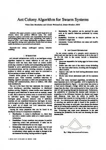
Figure 1, there is no aggregation nodes between the path from source 1 to the sink and the path from the source 2 to the sink (indicated in solid lines). If the search regions of the two paths are extended individually, the aggregation node G will be found and two new routing paths (indicated in dashed lines) will be formed.
Figure 1. The aggregation node G will be identified when the search regions are extended.
3.1 Next-Hop-Node Selection In WSNs, each sensor node has a unique identity. WSNs can be modeled by unit disk graph. A random unit disk graph G = (V, E) can be constructed. Place V nodes at random in a square area and connect with its neighbor at Euclidean distance less than or equal to transmission range R. Initially, every node has a pheromone table with its one-hop nodes. The pheromone of the path which does not deliver data gets evaporated with time. First, the sink will flood its identity to all nodes in networks. After the node receives this packet, it will compute the hop-count to the sink. As the source node wants to send data, it will select next hop node by following the probabilistic rule (see equation (1)) with which ant k as data packet in node i chooses to move to the node j until the sink node,
3. An Ant Algorithm for Data Aggregation In this section, we describe how to find aggregation points using an ant colony algorithm and illustrate how our proposed algorithm works. The proposed algorithm includes three steps. Step 1 is to select next hop node; step 2 is to extend the path around the node just selected; step 3 is to update the pheromone trails on neighboring nodes In paper [12], the probability to find aggregation nodes based on any two routing paths is not high. To increase the probability, this paper suggests extending the search region around the routing paths for finding out aggregation nodes in the network. For example, see
p k (i, j ) =
τ (i, j ) ×η (i, j )β β ∑τ (i, u )×η (i, u )
(1)
u∈N i
where τ is the pheromone, η is the inverse of the distance between node j and sink adding one, Ni is the number of neighbors of the node i, and β is a parameter which determines the relative importance of pheromone versus distance (β>0).
102
it will update its pheromone table according to equations (2), (3) and (4):
3.2 Producing Extended Paths After the node i selects its next hop node by applying equation (1), it sends a Select packet including the data packet to the next node. The Select packet consists six parts: z SN: selected node. z S: source id. z P: previous hop node id. z Dis: hop count from the node i to the source. z EHC: extended hop count. z TTL: time to live.
τ ij = (1 − ρ )τ ij + ρΔτ ij
[
(2)
]
Δτ ij = ζ +(hi −hj ) ×Δωj
Δω j = ∑ (H ij ) + (h j ) −1
−1
(3) (4)
i∈R j
where ρ is the pheromone decay parameter, ζ is a positive number, hi is the hop count between nodes i and sink, and hj is the hop count between nodes j and sink. In equation (3), if the value of (hi – hj) is greater than zero, it can conclude that node j is closer to the sink node than node i. Therefore, the algorithm will reward the path from node i to node j by depositing more pheromone. If the value equals to zero, it means that both nodes i and j have the same hop count to the sink, then the algorithm will lay little pheromone on the path. If the value is less than zero, the algorithm will not lay pheromone on this path. In equation (4), Rj is the set of sources through node j, and Σ(Hij)-1 is total hop number of these sources until node j. Therefore, Δωj is the total hop number of some sources to the sink through node j. The less the total hop number is, the more the amount of pheromone is added on the path from node i to node j, as shown in equation (3). This means that more ants will be encouraged to follow this path. For an aggregation node, it will update the pheromone levels of its all neighbors by the equation (2) when an ant moves to it. If a node does not have ants to visit it within a threshold time, its pheromone will be evaporated according to equation (5): (5). τ ij = (1 − ρ )τ ij
The field of Dis is computed by the hop count from the source to the node i. The initial value of Dis is zero. As the node j receives the Select packet, it will build a reaction table. The reaction table consists five parts: z S: source id. z P: previous hop node id. z Djs: hop count from the node j to the source. z EHC: extended hop count. z TTL: time to live. The S, P, EHC, and TTL of the reaction table are the same as those values in the Select packet. The Djs of the reaction table is the Dis of the Select packet adding one. Note that as the reaction table of a node has already existed, the node will check the S value of the Select packet with the S value of its reaction table. If both S values are the same, node j will update its reaction table by selecting the lower value of Djs; otherwise, it will add a new record for the Select packet. After node j has built or updated the reaction table, it will broadcast a new Select packet without the data packet to its neighbors. The SN of this packet is set to “*”, which means the one-hop broadcasting packet. The TTL of the Select packet is the TTL of the reaction table subtracting one. When the TTL value equals to 0, node j will stop its path extension.
After a short transitory period, the amount of pheromone of an aggregation node will be large enough to attract more ants carrying data packets from different sources to aggregate data. We will illustrate an example shown in Figure 2. Assume nodes A and B are source nodes and node D is a sink node. The sink node will flood its id to all nodes in the network. All nodes will compute the hop count to the sink as h. Suppose an ant on node A wants to transmit data, it will follow the probabilistic rule, equation (1), to selects next hop. In path I, node A sends a Select packet (C, A, A, 0, 1, 1) to node C. As node C receives the Select packet, it will build a reaction table as shown in Figure 3(a).
3.3 Pheromone Updating Rule As the EHC is equal TTL of the node’s reaction table, node j will send a Pheromone_Update packet to its parent, node i. The Pheromone_Update packet consists four parts: z ID: node id. z P: previous hop node id. z hj: hop count of the node j to sink z Δωj: total cost of some sources until the sink through node j. When node i receives a Pheromone_Update packet,
103
runs, the two final routing paths will be formed and aggregated at node G.
Figure 4. The node G broadcasts pheromone updating packets to its neighbors.
4. Simulation Results Figure 2. A network has two source nodes, A and B, and one sink node, D.
We first compared the performance of our algorithm performance with the DD method. For these simulation experiments, we assumed that there are sensor nodes distributed randomly in a square 100m×100m region. All nodes have the same transmission range. There is a single sink located at coordinate (10, 10) of the network which receives data of all source nodes for all simulations. We use an energy model [5] to estimate the power consumption. The energy consumption for sending a packet is determined by a cost function: Esend = Etrans * s + Eamp * d2, where Esend is the energy cost of sending a bit, s is the packet size, Eamp is the energy consumed in the amplifier, and d is the distance of message transmission. The energy consumption for receiving a message is determined by a cost function: Ereceive = Erec * r, where Etrans is the energy cost of receiving a bit, and r is the packet size.
The table includes the source id (S) = A, the previous hop node id (P) = A, the hop count from node C to the source node A is 1 (Djs= Dis + 1), the extended hop count (EHC) is 1, and the time to live (TTL) is 1. Then node C broadcasts a Select packet (*, A, C, 1, 1, 0) to its 5 neighbors. Node A (the current parent of node C) will ignore this packet. After that, node C will check that whether the EHC is equal to TTL. If the condition is true, node C will send a Pheromone_Update packet (C, A, hc,ΔωC) to node A. S
P
D js
EHC
TTL
A
A
1 (a)
1
1
S
P
D js
EHC
TTL
A
C
2 1 0 (b) Figure 3. (a) The reaction table of node C. (b) The reaction table of the neighbors of node C.
Table 1. Simulation Parameters.
Symbo l N S R Etrans Ereceive Eamp CPsize DPsize Senergy
In this example, the algorithm builds an extended routing paths for source A and B respectively, and there are some nodes such as F, G, and L (aggregation nodes) overlapped by the two extended routing paths. For aggregation nodes, they will send pheromone updating packets to their own neighbors to reinforce their relationships. In Figure 4, node G broadcasts Pheromone_Update packet (G, *, 2, ΔωG) to its neighbors E, F, J, L, K, and N. The values of hE, hF, hG, hJ, hL, hK and hN are 2, 1, 2, 3, 1, 2, and 3, respectively. Nodes E, F, J, L, K, and N will update their pheromone by equation (3). The increasing amount of pheromone of node J and N are Δτ JG = ζ +(3−2) ×ΔωG . Each ant will perform the same procedure (three steps) at each node on its constructed path. After many
[
ρ β
]
ζ
104
Definition
Setting
Number of sensor nodes Number of source nodes Transmission range Transmitter electronics Receiver electronics Transmit Amplifier Size of control packet Size of data packet Initial energy of sensor nodes Pheromone decay parameter Relative importance of pheromone versus distance A positive number
300 to 500 5 to 20 10m to 14m 50nJ/bit 50nJ/bit 0.1nJ/bit/ m2 One byte 64 bytes 0.25J 0.3 20 1
The third set of experiments is carried out for measuring the maximum run (lifetime) by comparing the DD method and the proposed algorithms with R=12. Figure 7 shows the results by varying the number of source nodes with N=300. It can be found that the maximum run of Ant-1 and Ant-2 are greater than Ant0 and DD. The reason is that Ant-1 and Ant-2 can find more aggregation nodes to share the same paths. In addition to that, the neighboring nodes of the sink node will receive aggregated data only, and thus they consume less energy.
The simulation parameters are given in Table 1. The simulation results presented here are the averages of 30 simulation runs. The first set of experiments is carried out for investigating the total energy consumption with N=300 and R=12. Figure 5 shows the results that apply directed diffusion (DD) and the proposed algorithms Ant-0, Ant-1, and Ant-2 with different EHC values: 0, 1, and 2, respectively. We also vary the number of source nodes to observe the behavior. Since the DD method does not perform data aggregation, it consumes much of energy. For the Ant-0 method, it generates fewer aggregation nodes than Ant-1 and Ant-2, so it costs more energy too. The Ant-1 and Ant2 methods consume less energy than the other two methods because they can find more nodes to aggregate data.
Figure 7. Runs vs. the number of source nodes for methods Ant-0, Ant-1, Ant-2 and DD.
The fourth experiment is to measure the total overhead and total transmitting amount of data with R=12 for 30 simulation runs. Besides the previous two methods, the GIT method is also considered for comparison. Figure 8 and Figure 9 show the results by varying the number of source nodes with N=400. In Figure 8, the GIT method broadcasts a lot of control packets to find shortest path to connect the established tree for each source at first run. Although each source only broadcast once, the total energy consumption is very high. In Figure 9, the GIT method uses a greedy method to find a shortest path with the established tree. Thus it consumes less energy for data transmission than Ant-0, but still higher than Ant-1 and Ant-2.
Figure 5. Total energy consumption vs. the number of source nodes for methods Ant-0, Ant-1, Ant-2 and DD.
The second experiment is to carry out for measuring the average energy consumption for each source node using the Ant-1 method with R=12 and N=400. Figure 9 shows the results by varying the number of source nodes in different run. In the first run, the aggregation does not happen, so the average energy consumption for one source node is almost equal for different number of source nodes. For the 30th run, the more the number of source nodes is, the more the number of aggregation nodes is, and thus the less the average consumed energy is.
Figure 8. Total energy consumption of overhead for different numbers of source nodes.
Figure 6. Average energy consumption for each source node by varying the number of source nodes in different run.
105
[2]
[3] Figure 9. Total energy consumption for data transmission for different numbers of source nodes. [4]
The Figure 10 demonstrates the final result of the proposed ant colony algorithm after 30 runs. It depicts the aggregation trees topology formation with N=400, S=10, and R=12. When the source nodes send out data packets at first run, the pheromone has not been accumulated on any node yet. Therefore, no data packet can be aggregated. After thirty runs, the aggregation tree is formed as shown in Figure 10, and data packets can be aggregated at 6 aggregation nodes.
[5]
[6]
[7]
[8] [9]
Figure 10. The aggregation tree constructed after 30 runs.
[10]
5. Conclusion This paper presents an ACO-based algorithm to perform data aggregation for wireless sensor networks with multiple source nodes and one sink node. After a short transitory period, the amount of pheromone on the aggregation nodes is sufficiently large to guide ants (the data packets from different sources) to meet together at these nodes for data aggregation. Simulation results show that the proposed algorithm actually consumes less data delivery energy than other traditional methods such as the DD and GIT methods.
[11]
[12]
[13]
6. References [1] Subhasis Bhattacharjee and Nabanita Das, “Distributed Data Gathering Scheduling in Multihop Wireless Sensor Networks for Improved Lifetime,” Proceedings of the
106
International Conference on Computing: Theory and Applications, Mar. 2007. Marco Dorigo and Luca Maria Gambardella, “Ant colony system: A cooperative learning approach to the traveling salesman problem,” IEEE Transactions on Evolutionary Computation, Volume 1, Issue 1, Apr. 1997. Frederick Ducatelle, Gianni Di Caro, and Luca Maria Gambardella, “Using ant agents to combine reactive and proactive strategies for routing in mobile ad hoc networks,” International Journal of Computational Intelligence and Applications, Vol. 5, No. 2, Mar. 2005. Anna Ha’c, Wireless sensor network designs, John Wiley & Sons Ltd, 2003. Wendi Rabiner Heinzelman, Anantha Chandrakasan, and Hari Balakrishnan, “Energy-Efficient Communication Protocol for Wireless Microsensor Networks,” Proceedings of the 33rd Hawaii International Conference on System Sciences, Jan. 2000. Chalermek Intanagonwiwat, Deborah Estrin, Ramesh Govindan, and John Heidemann, “Impact of density on data aggregation in wireless sensor networks,” Proceedings of the 22nd International Conference on Distributed Computing Systems, Nov, 2001. Chalermek Intanagonwiwat, Ramesh Govindan, Deborah Estrin, John Heidemann, and Fabio Silva, “Directed diffusion for wireless sensor networking,” IEEE/ACM Transactions on Networking, Vol. 11, No. 1, Feb. 2003. Mohammad Ilyas and Imad Mahgoub, Handbook of sensor networks, CRC Press, London, 2005. Bhaskar Krishnamachari, Deborah Estrin, and Stephen Wicker, “The impact of data aggregation in wireless sensor networks,” Proceedings of the 22nd International Conference on Distributed Computing Systems Workshops, Jul. 2002. Deying Li, Jiannong Cao, Ming Liu, Yuan Zheng, “Construction of Optimal Data Aggregation Trees for Wireless Sensor Networks,” Proceedings -15th International Conference on Computer Communications and Networks, Oct. 2006. Hong Luo, Yonghe Liu, and Sajal K. Das, “Routing correlated data with fusion cost in wireless sensor networks,” IEEE Transactions on Mobile Computing, Vol. 5, No. 11, Nov. 2006. Rajiv Misra and Chittaranjan Mandal, “Ant-aggregation: Ant colony algorithm for optimal data aggregation in wireless sensor networks,” Wireless and Optical Communications Networks IFIP International Conference, Apr. 2006. Shinji Motegi, Kiyohito Yoshihara and Hiroki Horiuchi, “DAG based In-Network Aggregation for Sensor Network Monitoring,” International Symposium on Applications and the Internet, Jan. 2006.