was rst presented in the context of electrical circuits analysis (Pen eld et al., 1970), nds applications in a ... in signal processing (Oppenheim and Schafer, 1989).
Relating Real-Time Backpropagation and Backpropagation-Through-Time: An Application of Flow Graph Interreciprocity. Fran�coise Beaufays and Eric A. Wan �
Abstract
We show that signal ow graph theory provides a simple way to relate two popular algorithms used for adapting dynamic neural networks, real-time backpropagation and backpropagation-through-time. Starting with the ow graph for real-time backpropagation, we use a simple transposition to produce a second graph. The new graph is shown to be interreciprocal with the original and to correspond to the backpropagation-through-time algorithm. Interreciprocity provides a theoretical argument to verify that both ow graphs implement the same overall weight update.
Introduction
Two adaptive algorithms, real-time backpropagation (RTBP) and backpropagation-throughtime (BPTT), are currently used to train multilayer neural networks with output feedback connections. RTBP was rst introduced for single layer fully recurrent networks by Williams and Zipser (1989). The algorithm has since been extended to include feedforward networks with output feedback (see, e.g., Narendra 1990). The algorithm is sometimes referred to as real-time recurrent learning, on-line backpropagation, or dynamic backpropagation (Williams and Zipser; Narendra et al., 1990; and, Hertz et al., 1991). The name recurrent backpropagation is also occasionally used, although this should not be confused with recurrent backpropagation as developed by Pinenda (1987) for learning xed points in feedback networks. RTBP is well suited for on-line adaptation of dynamic networks where a desired response is speci ed at each time step. BPTT, (Rumelhart et al. 1986; Nguyen and Widrow, 1990; and Werbos, 1990), on the other hand, involves unfolding the network in time and applying standard backpropagation through the unraveled system. It does not allow for on-line adaptation as in RTBP, but has been shown to be computationally less expensive. Both algorithms attempt to minimize the same performance criterion, and are equivalent in terms of what they compute (assuming all weight changes are made o�-line). However, they are generally derived independently and take on very di�erent mathematical formulations. In this paper, we use ow graph theory as a common support for relating the two algorithms. We begin by deriving a general ow graph diagram for the weight updates associated with � The authors are with the department of Electrical Engineering, Stanford University, Stanford, CA 94305-
4055. This work was sponsored by EPRI under contract RP8010-13.
1
RTBP. A second ow graph is obtained by transposing the original one, i.e., by reversing the arrows that link the graph nodes, and by interchanging the source and sink nodes. Flow graph theory shows that transposed ow graphs are interreciprocal, and for single input single output (SISO) systems, have identical transfer functions. This basic property, which was rst presented in the context of electrical circuits analysis (Pen eld et al., 1970), nds applications in a wide variety of engineering disciplines, such as the reciprocity of emitting and receiving antennas in electromagnetism (Ramo et al., 1984), the relationship between controller and observer canonical forms in control theory (Kailath, 1980), and the duality between decimation in time and decimation in frequency formulations of the FFT algorithm in signal processing (Oppenheim and Schafer, 1989). The transposed ow graph is shown to correspond directly to the BPTT algorithm. The interreciprocity of the two ow graphs allows us to verify that RTBP and BPTT perform the same overall computations. These principles are then extended to a more elaborate control feedback structure.
Network Equations
A neural network with output recurrence is shown in Figure 1. Let r(k ? 1) denote the vector of external reference inputs to the network and x(k ? 1) the recurrent inputs. The output vector x(k) is a function of the recurrent and external inputs, and of the adaptive weights w of the network: x(k) = N (x(k ? 1); r(k ? 1); w): (1)
r(k ? 1)
x(k)
N
x(k ? 1)
q Figure 1: Recurrent neural network (q represents a unit delay operator). The neural network N is most generally a feedforward multilayer architecture (Rumelhart et al., 1986). If N has only a single layer of neurons, the structure of Figure 1 represents a completely recurrent network (Williams and Zipser, 1989; Pineda, 1987). Any connectionist architecture with feedback units can, in fact, be represented in this standard format (Piche, 1993). Adapting the neural network amounts to nding the set of weights w that minimizes the cost function " # X 1 1 X E h e(k) e(k) i ; J = E e ( k ) e(k ) = (2) 2 2 =1 =1 K
K
T
T
k
k
2
where the expectation E [�] is taken over the external reference inputs r(k) and over the initial values of the recurrent inputs x(0). The error e(k) is de ned at each time step as the di�erence between the desired state d(k) and the recurrent state x(k) whenever the desired vector d(k) is de ned, and is otherwise set to zero: ( if 9 d(k) e(k) = d0 (k) ? x(k) otherwise (3) For such problems as terminal control (Bryson and Ho, 1969; Nguyen and Widrow, 1990) a desired response may be given only at the nal time k = K , while for other problems such as system identi cation (Ljung, 1987; Narendra, 1990) it is more common to have a desired response vector for all k. In addition, only some of the recurrent states may represent actual outputs while others may be used solely for computational purposes. In both RTBP and BPTT, a gradient descent approach is used to adapt the weights of the network. At each time step, the contribution to the weight update is given by h
i
e(k) e(k) dx(k ) = � e(k ) � ; �w(k) = ? 2 dw dw T
� d
T
T
(4)
where � is the learning rate. Here the derivative is used to represent the change in error due to a weight change over all time1. The accumulation of weight updates over k = 1:::K is P given by �w = =1 �w(k). Typically, RTBP uses on-line adaptation in which the weights are updated at each time k, whereas BPTT performs an update based on the aggregate �w. The di�erences due to on-line versus o�-line adaptation will not be considered in this paper. For consistency, we assume that in both algorithms the weights are held constant during all gradient calculations. K k
Flow Graph Representation of the Adaptive Algorithms
RTBP was originally derived for fully recurrent single layer networks2. A more general algorithm is obtained by using equation 1 to directly evaluate the state gradient dx(k) = dw in the above weight update formula. Applying the chain rule, we get: dx(k ) @ x(k ) dx(k ? 1) @ x(k ) dr(k ? 1) @ x(k ) dw = � + � + � dw ; (5) dw @ x(k ? 1) dw @ r(k ? 1) dw @w in which dr(k ? 1) = dw = 0 since the external inputs do not depend on the network weights, and dw = dw = I , where I is the identity matrix. With these simpli cations, equation 5 reduces to: dx(k ) @ x(k ) dx(k ? 1) @ x(k ) = � + : (6) dw @ x(k ? 1) dw @w We de ne the derivative of a vector a 2