AN APPROACH TO FULLY UNSUPERVISED HYPERSPECTRAL UNMIXING. Wolfgang Gross, Hendrik Schilling, Wolfgang Middelmann. Fraunhofer Institute of ...
AN APPROACH TO FULLY UNSUPERVISED HYPERSPECTRAL UNMIXING Wolfgang Gross, Hendrik Schilling, Wolfgang Middelmann Fraunhofer Institute of Optronics, System Technologies and Image Exploitation (IOSB), Gutleuthausstr. 1, 76275 Ettlingen, Germany ABSTRACT In the last few years, unmixing of hyperspectral data has become of major importance. The high spectral resolution results in a loss of spatial resolution. Thus, spectra of edges and small objects are composed of mixtures of their neighboring materials. Due to the fact that supervised unmixing is impossible for extensive data sets, the unsupervised Nonnegative Matrix Factorization (NMF) is used to automatically determine the pure materials, so called endmembers, and their abundances per sample [1]. As the underlying optimization problem is nonlinear, a good initialization improves the outcome [2]. In this paper, several methods are combined to create an algorithm for fully unsupervised spectral unmixing. Major part of this paper is an initialization method, which iteratively calculates the best possible candidates for endmembers among the measured data. A termination condition is applied to prevent violations of the linear mixture model. The actual unmixing is performed by the multiplicative update from [3]. Using the proposed algorithm it is possible to perform unmixing without a priori studies and accomplish a sparse and easily interpretable solution. The algorithm was tested on different hyperspectral data sets of the sensor types AISA Hawk and AISA Eagle. Index Terms— NMF, unmixing, endmember calculation, progressive OSP, fully unsupervised 1. BASICS OF SPECTRAL UNMIXING Airborne hyperspectral sensors are often used for large-scale mapping and classification. Their demand for high spectral resolution comes at the cost of spatial resolution. This results in spectra containing more than one material. Depending on the size and complexity of a data set it becomes increasingly difficult to select the endmember spectra manually. Choosing the wrong amount or unsuitable spectra results in an unmixing, which does not match the physical situtation. Several approaches exist, to automatically determine the spectra of pure materials and their fractions, so called abundances, in every sample. In this paper, only the assumption of linear mixtures is considered. In general, nonlinear ap-
proaches require widespread a priori information of the data set, which contradicts the demand for unsupervised unmixing. A comparison of several supervised nonlinear approaches can be found in [4]. In spectral unmixing, the measured samples of a hyperspectral data set are treated as high-dimensional feature vectors. The underlying optimization problem of the linear mixture model can be written as minW,H kV − W HkF , subject to W, H ≥ 0 per element. Here, V is the m × n data matrix with m bands and n samples, W is the m × k endmember matrix and H the k × n abundance matrix. All entries of the matrices are real and nonnegative numbers. To prevent undesired discrimination of the same material with different intensities, all spectra are normalized employing k·k1 . Normalization is also a prerequisite for the unsupervised initialization presented in the next section. However, it has to be noted that normalization can pose problems in conjunction with additive noise. After normalization, every spectrum is an element of the m − 1-dimensional hyperplane, which is a convex combination of the m Euclidean unit vectors. Usually, the inherent dimension of a data set is much smaller than m and a set of k vectors, with k � m can approximate the data very well [5]. In present approaches, the amount of endmembers used for unmixing has to be chosen previous to initialization and the methods to determine k are either very time-consuming (full unmixing with varying k) or cannot be mathematically motivated with regard to the nonnegativity constraint (e.g. scree test from Principal Component Analysis). A large amount of initialization methods for W can be found in [2], [6] and [7]. As none of these methods was able to find the actual endmembers in an ideal noiseless data set, another procedure has to be used. The initialization proposed in this paper is motivated by [8] and repeatedly performs OSP to determine the signatures with maximal distance to a certain seeding point, which in turn are vertices of the high-dimensional polygon described by the convex hull of the data set. Unmixing is performed, using the alternating multiplicative update rule from [3].
2. FULLY UNSUPERVISED UNMIXING The approach to fully unsupervised unmixing consists of three different steps and operates on k·k1 -normalized data. In Step 1, the best candidates for endmembers among the sample spectra are determined and the inherent dimensionality for the following steps is set. With the results, Step 2 computes the fractional abundances towards these candidates. In the last step, alternating optimization is performed to calculate the actual endmembers, which may not be apparent among the sample spectra and their corresponding abundances. Step 1: Initialization of W via progressive OSP: The m-dimensional hyperspectral sample vector w1 with maximal Euclidean distance to the first sample of the data set w0 is calculated. The first sample is chosen to eliminate random procedures. Whether the first sample lies in a region degraded by noise does not matter as it is discarded afterwards. Following this rule, results of unmixing processes are reproducible for each data set. Due to normalization, w1 is a guaranteed endmember in noiseless data. The next candidate w2 is chosen to be the sample with maximal distance to w1 . The new candidate w2 has to be on an extreme direction of the minimal convex cone containing the data. This is the best possible solution to determine the endmember candidates with respect to the measured data. Now, OSP is performed along the vector l1 connecting w1 and w2 . The projection matrix is calculated as the inner product of the transpose orthogonal subspace S 0 of l1 with the data matrix V . In S 0 , w10 and w20 have identical coordinates and the next candidate w3 is chosen, such that the line segment l20 = w20 w30 has maximal length and l2 = w2 w3 is saved along with l1 in the direction matrix L. The projection on the orthogonal subspace to L is repeated (i−1) iteratively. The longest line segments li are determined in S (i−1) , then the endmember wi+1 is identified in the original space and li = wi wi+1 is appended to L. The algorithm is terminated when one endmember candidate lies inside a low-intensity area like shadow or water. Further endmembers would only serve to approximate noise in the data. In the case of simulated noiseless data, the iteration is terminated, when the distance towards the next candidate drops below computation accuracy in the current subspace. Step 2: Initialization of H via projected fractions: The abundances in H are estimated by their fractional part, that is not accounted for by any other endmember. Each row Hi: of H is calculated separately by −i Hi: = wiT POSP , −i T T where POSP = (I − W−i (W−i W−i )−1 W−i )V , I is the unit matrix of suitable dimension and W−i is the endmember matrix W without the i-th endmember.
Step 3: Unmixing via alternating multiplicative update: Now, the alternating iteration from [3] is performed to optimize the results from the previous steps: H (t+1) = H (t) ∗
((W (t) )T V ) (W (t) )T W (t) H (t)
+�
(t+1) T
W (t+1) = W (t) ∗
(V (H ) ) W (t) H (t+1) (H (t+1) )T + �
Here, (t) is the iteration index and ∗ and ·· denotes multiplication/division per element. � is a small, strictly positive value to prevent division by zero. Iteration is terminated,
2 when the error gradient ∆(t) = V − W (t−1) H (t−1) −
V − W (t) H (t) 2 satisfies ∆(t) < δ, where δ is the tolerance threshold. Obeying the linear mixture model, Step 1 is concluded when a candidate is chosen on the border between two materials or inside an area of low-intensity. Thus, selection of material spectra dominated by noise is avoided. According to the theorem of intersecting lines, the effects of additive noise have greater impact in low-intensity regions, when normalization is performed. A pseudocode of Step 1 can be found in [9]. Step 2 is an analytical calculation and needs no separate termination condition. The alternating iteration in Step 3 should be terminated, when significant improvement can no longer be expected. One approach is to calculate ∆(t) and set δ = 100 ∗ ∆(t+100) . Thus, if the error gradient is less than a hundredth of the gradient calculated before, iteration stops. It is time-consuming to calculate ∆(t) , so checking for δ should only be done every 100 iterations. Also, the error gradient is very steep in the first iterations. To prevent early termination, the comparison should approximately start by calculating ∆(t) with t > 30. 3. EXPERIMENTAL RESULTS The algorithm was tested on several hyperspectral data sets depicting Berlin, Germany. The upper left image of image 1 shows an intensity image of one data set. Each endmember candidate, determined in Step 1 is marked by a white cross. The other images show five of the nine resulting abundances after Step 3 and can be identified with different materials. The upper right image shows asphalt. The two images in the middle row complement themselves by showing vegetation on the left and soil on the right. It is apparent, that soil is detected in areas dominated by low vegetation and grass, but not in tree regions. The lower left image depicts one of two metal abundances. Here, inherent sparseness of the algorithm becomes apparent and individual cars can be distinguished from the background. The last image depicts shadow regions. The algorithm minimizes the approximation error of the underlying optimization problem. Thus, there will always be an endmember trying to approximate noise. For interpretation,
Fig. 1. : Intensity image of the original data with endmember candidates; five of the nine abundance images (asphalt, vegetation, soil, one of two metal endmembers and shadow regions) this particular endmember and its abundance image should be dismissed. Further testing was done on simulated hyperspectral data. A set amount of k = 9 distinct spectra were chosen from a real hyperspectral data set with m = 235 bands and treated as endmembers. They were linearly combined to create mixed spectra with known abundances. Each simulated data set was extended by the pure form of its corresponding endmembers to test the performance of the algorithm in the ideal noiseless case. As the virtual dimension of the simulated data is k ≤ m, Step 1 finds the endmember spectra analytically and terminates, when the distance towards a new candidate drops below computational accuracy in the current subspace. After Step 2 is performed, only minor improvements occur through Step 3, as the alternating update already starts in the vicinity of an optimal solution and the data is not degraded by noise. Applying the algorithm to simulated noiseless data, a root mean squared error of 0.016 between actual and calculated abundances, subject to the sum-to-one constraint, was measured per sample.
In contrast to the initialization methods from [2], [6] and [7], no random procedures are used in Step 1, which results in reproducible unmixing. 4. CONCLUSIONS AND OUTLOOK The proposed fully unsupervised unmixing algorithm can be used without a priori knowledge of the data set and without specifying any parameters. It allows interpretation of hyperspectral data by reducing its dimensionality to the number of materials, which can be isolated above noise level. Additionally, no random procedures are employed in the algorithm, which prevents multiple unmixing solutions for the same data set. The initialization procedure in Step 1 calculates a lowdimensional convex cone, which best approximates the convex cone containing the convex hull of the sample spectra in high-dimensional space. According to the definition, the sample spectra on these vertices are called endmembers. In the noiseless case, every endmember is found, which is the prerequisite to achieving the best possible unmixing.
Step 2 initializes the abundances per endmember by calculating their fractional part, that is not accounted for by any other endmember. When the data contains noise, Step 3 further optimizes the results of the previous steps with respect to the underlying optimization problem by an alternating coordinate descent approach. New endmembers are calculated outside the convex hull of the original data set to account for variations in the separate material classes, abundances are optimized accordingly. In future works, robust algorithms to detect and correct lowintensity regions should be developed. This includes measuring their dependency on calibration and sensor specific behavior. Also, an adaptive termination condition for step 3, solely depending on the amount of endmember candidates and the data, should be examined.
5. REFERENCES [1] S. Wild, J. Curry, and A. Dougherty, “Motivating nonnegative matrix factorizations,” SIAM, vol. 8, 2003. [2] A. Langville, C. Meyer, and R. Albright, “Initializations for the nonnegative matrix factorization,” Proceedings of the Twelfth ACM SIGKDD International Conference on Knowledge Discovery and Data Mining, 2006. [3] D. Lee and H. Seung, “Algorithms for non-negative matrix factorization,” vol. 13, pp. 556–562, 2001. [4] W. G. Liu and E. Y. Wu, “Comparison of non-linear mixture models: Sub-pixel classification,” Remote Sensing of Environment, vol. 94, no. 2, pp. 145–154, 2005. [5] C. Chang and Q. Du, “Estimation of number of spectrally distinct signal sources in hyperspectral imagery,” vol. 42, no. 3, pp. 608–619, 2004. [6] Y. Masalmah and M. Velez-Reyes, “The impact of initialization procedures on unsupervised unmixing of hyperspectral imagery using the constrained positive matrix factorization,” Proc. SPIE 6565, vol. 6565B, 2007. [7] S. Wild, J. Curry, and A. Dougherty, “Improving nonnegative matrix factorizations through structured initialization,” Pattern Recognition, vol. 37, no. 11, pp. 2217– 2232, 2004. [8] C. Chang, “Orthogonal subspace projection (osp) revisited: A comprehensive study and analysis,” IEEE Trans. Geosci. Remote Sens., vol. 43, no. 3, pp. 502–518, 2005. [9] W. Gross and W. Middelmann, “Sparseness inducing initialization for nonnegative matrix factorization in hyperspectral data,” Proc. 32. Wissenschaftlich-Technische Jahrestagung der DGPF, vol. 21, pp. 306–313, 2012.