text of performance problems in the CPU and paging sub-systems of a production ... commonly, detection is done by monitoring measure- ment variables (or ...
An Approach to Selecting Metrics for Detecting Performance Problems in Information Systems Proceedings of the Second International Conference on Systems Management June 19-21, 1996 Toronto, Canada Joseph L. Hellerstein IBM Research Division T.J. Watson Research Center Yorktown Heights, New York 10598
Abstract
Abstract
Early detection of performance problems is essential to limit their scope and impact. Most commonly, performance problems are detected by applying threshold tests to a set of detection metrics. For example, suppose that disk utilization is a detection metric, and its threshold value is 80%. Then, an alarm is raised if disk utilization exceeds 80%. Unfortunately, the ad hoc manner in which detection metrics are selected often results in false alarms and/or failing to detect problems until serious performance degradations result. To address this situation, we construct rules for metric selection based on analytic comparisons of statistical power equations for ve widely used metrics: departure counts (D), number in system (L), response times (R), service times (S ), and utilizations (U ). These rules are assessed in the context of performance problems in the CPU and paging sub-systems of a production computer system.
1 Introduction
Complex information systems require early detection of performance problems in order to limit the problem's impact and to simplify its resolution. Most commonly, detection is done by monitoring measurement variables (or metrics) that are compared to threshold values. An alarm is raised if a threshold is violated. For example, suppose that disk utilization is a detection metric, and its threshold value is 80%. Then, an alarm would be raised if disk utilization exceeds 80%. Today's network management systems typically employ hundreds of such detection metrics. Unfortunately, there is little understanding of when one detection metric is preferred to another, and so the selection of detection metrics is fairly ad hoc. As a result, alarms are frequently raised when no performance problem is present, and many problems are not detected until serious performance degradations result. Herein, we take a step towards improving this
situation by using simple analytic models to construct rules for selecting detection metrics. These rules are assessed in the context of three performance problems in a production computer system. Our focus is interactive performance because of its relationship to end-user productivity as well as to other quality of service considerations. We view an information system as a network of queues. As such, a performance problem is an adverse impact on interactive performance that results from changes in queueing parameters, such as increases in expected arrival rates or larger expected service times. Examples of performance problems include: increased network tra�c due to adding a le server to a local area network; slower service rates due to intermittent disk failures; and increased service times due to changes in application software. We consider ve metrics for detecting performance problems: departure counts (D), number of customers in the system (L), response times (R), service times (S), and utilizations (U). (The D metric is based on measurements taken over an interval of length T.) Choosing detection metrics and their threshold values should be done with two objectives in mind. First, false alarms should be infrequent. That is, it should be rare that a threshold is violated when no performance problem is present. Second, power should be high. That is, there should be a high probability of a threshold violation when a performance problem is present. Not surprisingly, there is a trade-o� between these two objectives. Changing threshold values so as to lower false alarms typically lowers power, and changing threshold values so as to increase power usually increases false alarms. Why not select as the detection metrics those measurement variables that estimate values of the queueing parameters that characterize performance problems? There are several reasons why this cannot or should not be done. First, the required measurement variables may not be available. For example, the UNIXTM system activity reporter (sar) does not
2 Selecting Detection Metrics
report service time or transaction rate information. Second, even if the necessary measurements can be obtained, making them available may be undesirable because monitoring the large number of hardware and software queues in production computer systems (especially networked information systems) means that massive volumes of data must be collected, stored, and processed. Third, even if the necessary measurements are available, having separate tests for each queueing parameter can greatly increase the number of false alarms. That is, there may be a high probability that at least one threshold will be violated when no performance problem is present. Fourth, it turns out that estimators of a queueing parameter may not provide the most powerful test for performance problems characterized by changes in that parameter. For example, we show that an increase in expected service times is, in some situations, more readily detected by using response time metrics rather than by using measured service times. Detection may be done either o�-line or on-line. In o�-line detection, data are presented en mass. In online detection, measurement variables are monitored continuously. Our focus is o�-line detection, although it turns out that metrics that provide powerful o�line detection can also be e�ective at on-line detection (e.g., the Shewhart algorithm [1]). From our de nition of a performance problem and based on the nature of the metrics studied, threshold comparisons have the form X� > CX . Here, X� is the sample mean of the metric X, and CX is chosen based on the level of false alarms that is considered acceptable. The topic of selecting threshold values for detection metrics is of great concern in operational settings (e.g., [8] and [5]), especially for large, distributed information systems. However, little attention has been paid to comparing detection metrics. Indeed, we are aware of only one study that addresses such comparisons [2]. Unfortunately, this study is limited in that: (a) it only considers departure rates, queue lengths, and response times; and (b) it does not consider false alarms or statistical power. There is a well developed theory of statistical hypothesis testing that provides a formal approach to analyzing both o�-line detection (e.g., [7]) and on-line detection (e.g., [1]). Indeed, we use the theory of o�-line detection in our analysis. However, this literature focuses on the statistics employed (e.g., the use of the sample mean versus its median), not on the choice of detection metric (e.g., comparing the power of R and L). Last, there is a general theory for both o�-line and on-line detection of changes in process control systems [1]. While this theory addresses non-linear systems in general, we are unaware of the theory being applied to queueing systems in particular. The remainder of this paper is organized as follows. Section 2 uses simple analytic models to construct rules for selecting detection metrics. Section 3 evaluates these rules in the context of three performance problems in a production computer system. Section 4 addresses hybrid tests and queueing networks. Our conclusions are contained in Section 5.
This section constructs rules for selecting detection metrics. Subsection 2.1 uses M/M/1 queueing systems to build simple analytic models for the power of the metrics D, L, R, S, and U. Subsection 2.2 uses these models to construct selection rules. At the end of this section, we discuss the robustness of these rules to deviations from the M/M/1 assumptions.
2.1 Models
Our analysis of detection metrics is based on the theory of statistical hypothesis testing (e.g., [7]). We apply this theory to stable M/M/1, rst-come- rstserved (FCFS) queueing systems. Statistical hypothesis testing addresses how to choose between two hypotheses (or alternatives). In our study, these hypotheses are: � H (null hypothesis): No problem is present. � H 0 (alternative hypothesis): A problem is present. For an M/M/1 queueing system with a single customer class, it su�ces to consider an increase in expected arrival rates and/or an increase in expected service times. The expected arrival rate 0parameter0 is denoted by � when H holds and by � when H holds. Similarly, s and s0 are used for H and H 0. From our de nition of0a performance it must 0 > problem, be true that either � > � or s s, or both. Let � = �s and �0 0 = �0 s0 be the expected utilization when H and H hold, respectively. Since we limit ourselves to stable queueing systems, �; �0 < 1. Let X� be the sample mean of observations of the metric X. Then, E(U� j H) = � and E(U� j H 0) = �0 . Also, E(D� j H) = �T, E(D� j H 0) = �0T, E(S� j H) = s, and E(S� j H 0 ) = s0 . Let �X be the population mean of X under H. Note that for the metrics we study, �X is a function of � and s (and T in the case of departure counts). Similarly, let �0X be the population mean of X under H 0; �0X is a function of �0 and s0 (and T for D). For the metrics herein considered, the population mean is non-decreasing in expected arrival rates, expected service times, and T. Thus, by choosing X as a detection metric, we are implicitly postulating the following statistical hypotheses: � H: X� has mean �X (no problem is present) � H 0 : X� has mean �0X (a problem is present) with �0X > �X . For an ideal detection metric, �0X ? �X is large (and the0 variance of X is small). Clearly, the magnitude of �X ? �X depends on the metric and the nature of the performance problem. Indeed, in some situations, this di�erence may be negative (which indicates that X is not sensitive to the performance problem). For example, a small increase in expected service times in combination with a moderate decrease
2
where �[z] is the cumulative distribution function for the standard normal (mean 0 and variance 1), �?1[1 ? �] is the 1 ? � quantile of the standard nor� AX mal, and �X AX is the standard deviation of X. (which is de ned shortly) is a standard deviation adjustment factor for the metric X. AX accounts for batching and autocorrelations when X has the H distribution. We calculate power as �X = P(X� > CX j H 0 ) = 1 ? P(X�� �0 CX j H 0) 0 = 1 ? P( X�0?A�0 � C�0 ?A�0 j H 0 ); where A0X is the standard deviation adjustment factor for X under the H 0 distribution. Thus, �X = 1 ? �[?KX ] = �[KX ]: We refer to KX as the power term for X, where 0 KX = ��0 ?AC0 (2) ?1 0 = (� ?� )?(��0 AA0 )(� [1?�]) : Given the metrics X and Y , KX < KY is equivalent to �X < �Y . Also, observe that multiplying a metric by a constant has no e�ect on KX since the mean and standard deviation of X� are multiplied by the same constant. A consequence of this last observation is that departure counts (D) and departure rates (D=T) have the same power if T is constant. To calculate the standard deviation adjustment factors, we must consider two levels of batching. The rst level of batching (which is mostly of concern for L, R, S, and U) is done by the measurement collection facility: Individual samples are accumulated to form observed values. For example, in our case studies, queue lengths are sampled every second over 30 second measurement intervals. An observed value is an average of these 30 samples. The second level of the batching occurs when observed values are averaged to ensure independence. Let bX be the size of a rst level batch, BX be the size of a second level batch, and NX be the number of second level batches. That is, the measurement facility takes bX BX NX samples and reports BX NX observations that we form into NX batches to ensure independence. Let X(i; j) be the i-th sample in the j-th observation of the metric X. By assumption, the X(i; j) are identically distributed (but not necessarily independent) with variance �X2 . Note that the i-th observation is the mean P of the i-th rst-level batch and is computed as bj X(i; j)=bX . Let r1;n be the expected value of the lag n autocorrelation for the samples taken by the measurement facility. We want to know �12;X , the variance of an observed value of X. From [10], � � 2 1 + 2 Pb ?1 (b ?n)r1 � X n=1 b : �12;X = bX
in expected0 arrival rates causes the di�erence in utilizations (�U ? �U ) to be negative. (Such a situation arises in our case studies.) It turns out that if the observations of X are independent and identically distributed as normal random variables, then X� > CX is a most powerful test for deciding between H and H 0 [7]. CX is called � and is chosen so that the the critical value of X, probability of a false alarm (or Type I error) is no greater than a previously speci ed value, which is denoted by �. That is, CX is chosen so that � = P(X� > CX j H). The power of the X� > CX test is the probability of detecting a performance problem when one is present. Power1 is denoted by �X , where �X = P(X� > CX j H 0). Let Y be a second metric (e.g., L) with sample mean Y� . As with X, we use a test of the form Y� > CY . Because of the trade-o� between false alarms and power, comparisons between �X and �Y should be done when CX and CY are chosen so that P(Y� > CY j H) = � = P(X� > CX j H). Under these circumstances, we say that Y is more powerful than X if �Y > �X . That is, for the same level of false alarms, the probability that Y detects a performance problem is greater than the probability that X detects a performance problem. To proceed further, we make two assumptions. First, we assume that the central limit theorem (CLT) can be invoked to exploit the normal distribution. The CLT requires that samples be independent and identically distributed (iid) and that the sample size be large enough so that the limiting results hold. We assume that samples of a metric are identically distributed since this consideration is routinely handled in practice (e.g., by taking measurements at the same time of day over successive days). To ensure independence, observations are batched to remove autocorrelations. The guidelines in [7] can be used to ensure that the sample size is su�ciently large for the CLT to hold. Second, our analysis assumes that �, s, �0 , and s0 are known, although they may have arbitrary values (subject to the stability constraint). Doing so simpli es our analysis since we need not consider estimators of population variances. Of course, variance estimators are required in practice, as is done in our case studies. Thus, it is important to know the e�ect of these estimators on the relative power of metrics. We view this as an area in which further work is needed. We now show how to compute critical values (CX ) and power (�X ) under the assumption that X� is normally distributed0 with a known mean and variance under H and H . From [7],
? � CX = �X + (�X AX ) �?1 [1 ? �)] ;
X
X
X
X
X
X
X
X
X
X
X
X
X
X
X
X
X
X
(1)
1 To simplify the concepts and notation employed, we have deviated somewhat from standard terminology for statistical hypothesis testing. Technically, power is the probability of rejecting H , regardless of whether H or H holds. The de nition of power used in this paper is actually 1 ? , where is the probability of a false negative or Type II error. 0
X
X
;n
X
3
D
C �T + �T(�?1 [1 ? �])AD
L
p� � ?1 (1?�) + (1?�) (� [1 ? �])AL
(�0 T ?�T )?pp�T (�?1 [1?�])A �0 TA0 (�0 ?�)?pp�(1?�0 )(�?1 [1?�])A �0 (1?�)A0
R
s s ?1 (1?�) + (1?�) (� [1 ? �])AR
(s0 (1?�)?s(1?�0)0 )?s(1?0�0 )(�?1 [1?�])AR s (1?�)AR
S
s + (s)(�?1 [1 ? �])AS
(s0 ?s)?(s)(�?1[1?�])AS s0 A0S
Metric
U
K
p
D
p � + �(1 ? �)(�?1 [1 ? �])A
D
L
L
p
(�0 ?�)? p�(1?�)(�?1 [1?�])A
U
�0 (1?�0 )A0
U
U
Figure 1: Critical Values (C) and Power Terms (K) for M/M/1, FCFS A similar equation can be written to compute the variance of a second level batch from r2;n (the expected value of the lag n autocorrelation between observed values), �12;X , and BX . So, the standard deviation adjustment factor of X� is (3) AX = (AX (bX ; r1))p(AX (BX ; r2)) ; N where
v � Pb ?1 (b u u 1 + 2 n=1 t AX (bX ; r1) = bX X
X
;n
�
X
v � PB ?1 (B u u 1 + 2 n=1 t AX (BX ; r2) = BX X
?n)r1 b
Thus, assuming that the standard deviation adjustment factors for D and S are not very much smaller than those of the other metrics, we propose the following rules: � Rule 1: D is a poor choice for performance problems dominated by an increase in expected service times. � Rule 2: S is a poor choice for performance problems dominated by an increase in expected arrival rates. In the sequel, we do not consider D. Given this and based on the data collected in the case studies in Section 3, it seems reasonable to assume that AX = AY and A0X = A0Y . We proceed with pair-wise comparisons of the nonD metrics. Consider the choice between L and U. From KU and KL , it is clear that neither is a good choice if �0 < � since their K values are negative and hence power is low. Suppose instead that �0 � �. Then, it turns out that �L � �U for small increases in expected utilization. (For large increases in expected utilizations, both metrics have a large power.) To see this, let numr(KX ) be the numerator of the metric X in Fig. 1, and let denom(KX ) be its denominator. We show that numr(KL ) � numr(KU ), and denom(KL ) � denom(KU ). The comparison between numerators can be written as p ?p�(1 ? �0 ) � ? �(1 ? �):
X
?n)r2 B
;n
�
X
A0X is computed in the same manner. Computing CX and KX for the ve metrics we study only requires substituting the means and variances of these metrics into Eq. (1) and Eq. (2). The metric means and variances as reported in [6]. Fig. 1 contains the results of making the necessary substitutions.
2.2 Relative Power of Metrics
We use the analytic models in Fig. 1 to compare the power of the metrics D, L, R, S, and U. From these comparisons, rules are constructed for selecting detection metrics. We begin with a couple of observations about the models in Fig. 1. First, note that KD is not a function of s0 . Hence, D is insensitive to performance problems that consist only of an increase in expected0 service times. Similarly, KS is not a function of � . So, S is not sensitive to increases in expected arrival rates.
p
holds when This is equivalent to 1 p� 1?1?�0� , which p 0 0 0 � � � since 1 ? � � 1 ? � � 1 ? �. For the denominators, denom(KL ) � denom(KU ) is p�0 (1 ? �) � p�0 (1 ? �0 ): This is equivalent to �0 ?� � �(1?�). That is, for small increases in expected utilization, �L � �U . Thus, 4
� Rule 3: L is preferred to U (if standard deviation
Later on, we qualify Rule 6 somewhat since it is sensitive to service time distributions. We present one nal rule. Consider the comparisons of �L and �R in Rule 4 and Rule 5. The analysis used to establish these p rules is based on two inequalities: p� � 1 and �0 � 1. These inequalities suggest that �L � �R at high utilizations. Hence, we propose: � Rule 7: L and R are comparable choices at high utilizations (if standard deviation adjustment factors are equal). Fig. 2 summarizes the metric selection rules constructed in this section. For simplicity, equal standard deviation adjustment factors are assumed throughout even though the requirements for Rule 1 and Rule 2 are less stringent. How robust are these rules to deviations from the M/M/1 assumptions? Rule 1 and Rule 2 seem fairly robust, as long as service times and interarrival times are mutually independent and do not depend on the scheduling policy. In contrast, Rule 6 is not particularly robust. This rule favors R over S for performance problems dominated by an increase in expected service times. However, the rule depends strongly on the variance of S. For example, consider a queueing system with constant service times and a performance problem that is dominated by an increase in expected service times. Here, �S = 1 since KS = 1. Thus, Rule 6 is quali ed by a statement about the variance of S. Robustness considerations for the other rules are more di�cult to assess. For example, the choice between L and U in Rule 3 is a�ected by the distribution of interarrival and service times as well as scheduling policies. Consider an M/G/1 queue. �U is insensitive to the service time distribution and to scheduling policies. However, the mean and variance of L increase with the variance of the service time distribution. Also, scheduling policies such as last-come- rstserve have higher variance than rst-come- rst-serve. All of these factors a�ect �L . Similar considerations are present for Rules 4, 5, 6, and 7. Nevertheless, studies that we have done for M/G/1 queueing systems have produced results consistent with Rule 3 through Rule 7 (with an appropriate caveat about the variance of S in Rule 6). Even so, data from production systems are needed to understand how these rules fare in practice. Several of the selection rules hold only for certain kinds of performance problems. For example, Rule 1 and Rule 4 apply only if the performance problem is dominated by an increase in expected arrival rates. Unfortunately, prior knowledge of performance problems is rarely available in practice. However, by selecting detection metrics that jointly cover many kinds of performance problems, we can construct a hybrid test that is reasonably powerful for a broad range of performance problems. Hybrid tests are discussed in Section 4.
adjustment factors are equal). We now turn to the choice between L and R. Suppose that the performance problem consists only of an increase in0 expected arrival rates. For simplicity, let s = 1 = s . Substituting into KR in Fig. 1 yields ? � (�0 ? �) ? (1 ? �0 ) �?1[1 ? �] AR : (1 ? �)A0R Letting numr(KR ) and denom(KR ) refer to this equation, numr(KL ) � numr(KR ) is equivalent to ?p�(1 ? �0 ) � ?(1 ? �0 ): This is the same as p� � 1, which holds for stable queueing systems. Also, denom(KL ) � denom(KR ) is equivalent to p�0 (1 ? �) � (1 ? �); p or �0 � 1. Hence, � Rule 4: L is preferred to R for performance problems dominated by an increase in expected arrival rates (if standard deviation adjustment factors are equal). Now suppose that the performance problem consists only of an increase in expected service times. For simplicity, � = 1 = �0 . It turns out that under these conditions, �R � �L. We proceed as with Rule 3. Substituting into KR in Fig. 1 results in ? � (�0 ? �) ? �(1 ? �0 ) �?1[1 ? �] AR : �0 (1 ? �)A0R Let numr(KR ) and denom(KR ) refer to this equation. Note that numr(KR ) � numr(KL ) since ?�(1 ? �0 ) � ?p�(1 ? �0 ); or p� � 1. Similarly, denom(KR ) � denom(KL ) holds since p �0 (1 ? �) � �0 (1 ? �); p which is the same as �0 � 1. Thus, we propose � Rule 5: R is preferred to L for performance problems dominated by an increase in expected service times (if standard deviation adjustment factors are equal). Also, it turns out that R is more powerful than S. This is easily seen by repeating the above analysis for KR and KS , which results in the inequalities �0 � 0 and � � 0. So, � Rule 6: R is preferred to S for performance problems dominated by increases in expected service times (if standard deviation adjustment factors are equal).
3 Case Studies
This section uses performance problems in a production computer system to provide a real-world assessment of the metric selection rules in Fig. 2. These
5
For equal
standard deviation adjustment factors: � � � � � �
Rule 1: D is a poor choice for performance problems dominated by an increase in expected service times. Rule 2: S is a poor choice for performance problems dominated by an increase in expected arrival rates. Rule 3: L is preferred to U. Rule 4: L is preferred to R for performance problems dominated by an increase in expected arrival rates. Rule 5: R is preferred to L for performance problems dominated by increases in expected service times. Rule 6: R is preferred to S for performance problems dominated by increases in expected service times (if the variance of S is not too small). � Rule 7: L and R are comparable choices at high utilizations. Figure 2: Rules for Selecting Detection Metrics (From M/M/1, FCFS Queueing Systems)
performance problems occur in the CPU and paging sub-systems, which bear little resemblance to the M/M/1 queueing systems used to develop the metric selection rules. Nevertheless, the relative sensitivity of metrics to performance problems in the case studies is consistent with our selection rules. The case studies were obtained from a large time sharing system running the IBM VM/SP HPO Operating System [4] at a major telephone company. The workload is a mixture of text processing, scienti c applications, and program development. Performance problems were detected by user complaints, usually in the form of an irate phone call. Upon receipt of a complaint, the operations sta� collected measurement data, characterized the problem, and then took appropriate corrective actions. The operations sta� had great interest in identifying good detection metrics so that future performance problems could be identi ed early and resolved before end-users complained. Three performance problems are studied. The rst two relate to the CPU sub-system. This sub-system can be characterized as a two server queue with a complex, deadline scheduler. The third performance problem relates to the paging sub-system, a complex queueing network of input/output processes, controllers, and disk drives. The performance problems are summarized below: � Problem 1: Increased CPU service times due to an ine�ciently programmed application. � Problem 2: Increased CPU service times due to an operating system bug. � Problem 3: Increased paging rates due to an operating system bug. From the foregoing descriptions, it seems reasonable that Problem 1 and Problem 2 are dominated by an increase in expected services times, and Problem 3 is dominated by an increase in expected arrival rates.
Five data sets are used in our study. There is one data set for each of the problems, and separate reference data sets are used to establish baseline values for measurement variables in the CPU and paging subsystems. There are 10 observations in the Problem 1 data set; all other data sets contain 120 observations. Observed values of queue lengths, response times, service times, and utilizations are based on one-second samples that are averaged over thirty second intervals. Departure rates are obtained by accumulating departure counts over the a thirty second interval and then dividing by thirty to obtain a rate. (From Section 2, we know that the power of departure rates is the same as that for departure counts as long as T is constant.) From the foregoing, T = 30. For departure rates, bX = 1; for all other measurement variables, bX = 30. For the CPU problem, measurement variables were collected that correspond to each of the ve detection metrics considered in this paper: QDROPS, departure rate from the CPU queue (D=T); CPUQ, number of transactions waiting for or being served by the CPU sub-system (L); CPUR, response time for CPU transactions (R); CPUS, CPU service time (S); and SYSTCPU, the CPU utilization in percent (U). (Since there are two CPUs, 0 � SY STCPU � 200.) Data for the paging sub-system is more sparse. The variables reported are: PREAD, departure rate from the paging sub-system (D=T); PAGEQ, number of transaction waiting for or receiving service from the paging sub-system (L); and PAGER, response time to page-in requests (R). Fig. 3 displays descriptive statistics for the observations reported by the measurement facility. Included are mean values, lag 1 autocorrelations, and standard deviations for both (which appear after the �). Standard deviations for autocorrelations are obtained by using the Bartlett bound [9] (which, for the rst lag, is a function only of the sample size). Note that 6
Variable
Problem 1
Mean QDROPS 20.97 � 2.26 CPUQ 2.5 � 2.42 CPUR 0.126 � 0.133 CPUS 7.59 � 0.57 SYSTCPU 158.08 � 8.45 Variable
Mean
Problem 2
ACR Mean 0.35 � 0.32 25.06 � 2.25 0.24 � 0.32 2.83 � 3.03 0.30 � 0.32 0.116 � 0.129 0.32 � 0.32 7.37 � 0.54 0.19 � 0.32 183.65 � 9.48
Problem 3
ACR
CPU Reference Data
ACR 0.37 � 0.091 0.26 � 0.091 0.25 � 0.091 0.53 � 0.091 0.45 � 0.091
Mean 26.73 � 1.80 1.93 � 2.12 0.072 � 0.08 7.363 � 0.438 196.12 � 6.64
ACR 0.35 � 0.091 0.37 � 0.091 0.38 � 0.091 0.19 � 0.091 0.47 � 0.091
Paging Reference Data Mean
ACR
PREAD 69.77 � 13.52 0.405 � 0.091 68.92 � 13.98 0.277 � 0.091 PAGEQ 2.56 � 1.91 -0.134 � 0.091 1.46 � 1.19 0.023 � 0.091 PAGER 0.038 � 0.035 -0.178 � 0.091 0.021 � 0.018 0.055 � 0.091
� ACR: lag 1 autocorrelation. � u � v: u is the estimate and v is its standard deviation Figure 3: Descriptive Statistics for Observed Values in the Case Studies AD , A0D Estimates QDROPS CPU Reference .139 (AD0 ) QDROPS Problem 1 .316 (AD0 ) QDROPS Problem 2 .141 (AD ) PREAD Page Reference .132 (AD0 ) PREAD Problem 3 .152 (AD ) Figure 5: Standard Deviation Adjustment Factors for D Variables in the Case Studies
QDROPS and SYSTCPU are smaller in the Problem 1 and Problem 2 data than they are in the CPU reference data. This suggests that the performance problem combines an increase in expected service times with a decrease in expected arrival rates. Our analysis of the case study data relies on statistical techniques that require iid (independent and identically distributed) observations. In particular, we are concerned about autocorrelations in the measurement data. In the Problem 1 data set, there are seemingly large autocorrelations. However, all autocorrelations lie within (or very close to) one standard deviation of zero and so are not statistically signi cant. The other data sets do contain signi cant autocorrelations. These are removed by batching with a batch size of 12. Thus, in the Problem 1 data set, BX = 1 and NX = 10; in the other data sets, BX = 12 and NX = 10. We now quantify the relative sensitivity of the measurement variables to the performance problems in the case studies. To this end, we examine the di�erence between the variable's value in the performance problem and its value in the reference data. In all cases, a large di�erence means that the measurement variable is more sensitive to the performance problem (since we are detecting larger values of expected service times and expected arrival rates). The statistical signi cance of this di�erence is gauged by using a one-sided t-statistic (with care in computing the pooled variances when batch sizes di�er [3]). A larger t-statistic means greater sensitivity to the presence of a performance problem. Sensitivity can also be quanti ed using signi cance levels. This is the probability of a obtaining a test statistic larger than the one measured if the two populations are in fact identical. Thus, a small signi cance level indicates a sensitive measure-
Variable
Data Set
ment variable. Fig. 4 reports the results. The relative sensitivity of the measurement variables is almost the same in both of the CPU performance problems. In order of ascending value of signi cance levels (or descending values of t-statistics), this is CPUR, CPUS, CPUQ, QDROPS, and SYSTCPU for Problem 1. The positions of CPUS and CPUQ are reversed in Problem 2. For the paging performance problems, the variables are ordered as PAGEQ, PAGER, and PREAD. How do these results compare with the metric selection rules in Fig. 2? To assess this, we must consider the standard deviation adjustment factors. Standard deviation adjustment factors for the D variables (i.e. QDROPS and PREAD) can be estimated from Eq. (3), where bX = 1 and NX = 10. In the Problem 1 data set, BX = 1, and the r2;n are assumed to be zero (because they are not statistically signi cant). In the other data sets, BX = 12, and the r2;n are estimated from the measurement data (as in [9]). Fig. 5 displays the resulting estimates for the standard deviation adjustment factors. Note that with the exception of the Problem 1 data set (which has a much smaller sample 7
CPU Variable
Metric Type Problem 1
Page Variable
Metric Type Problem 3
QDROPS CPUQ CPUR CPUS SYSTCPU PREAD PAGEQ PAGER
D L R S U
D L R
0.99 (-7.49) 0.24 (0.71) 0.11 (1.25) 0.13 (1.17) 0.99 (-13.65)
Problem 2
0.99 (-4.02) 0.05 (1.68) 0.03 (2.03) 0.49 (0.03) 0.99 (-6.62)
0.38 (0.31) 0.000037 (5.10) 0.00015 (4.44)
� Entries have the form u (v): u is signi cance level; v is the t-statistic � A more sensitive test is indicated by a smaller signi cance level or a larger t-statistic. Figure 4: Signi cance Levels and t-statistics in the Case Studies size), the estimates are clustered around .141. Unfortunately, we lack the data necessary to estimate the other standard deviation adjustment factors in that we do not know the autocorrelations for the individual samples within a measurement interval. However, since the D standard deviation adjustment factors are approximately equal, it may be that the non-D standard deviation adjustment factors are equal as well. This suggestion is given further strength by noting that within each data set, the nonD variables (a) have the same bX , BX , and NX values and (b) have autocorrelations that lie within approximately two standard deviations of one another (although CPUS has somewhat more extreme autocorrelations). In the sequel, we assume that within each data set the standard deviation adjustment factors are equal for the non-D metrics. We begin with Rule 1: D is a poor choice if the performance problem is dominated by an increase in expected service times. Rule 1 is violated when T is quite large and/or when D's standard deviation adjustment factor is quite small. In the case study, T is moderate (i.e., 30). Further, the autocorrelations reported for the D variable in the CPU data (i.e., QDROPS) are within two standard deviations of the autocorrelations of the non-D variables. This observation suggests that the standard deviation adjustment factor for QDROPS is comparable to or larger than the standard deviation adjustment factor of the other CPU variables (since bD = 1). Hence, Rule 1 should apply. Indeed, the .99 signi cance level for QDROPS (D) in Fig. 4 is consistent with Rule 1. We expect D metrics to do better when the performance problem is dominated by an increase in expected arrival rates. This is consistent with PREAD having a signi cance level in the paging data set that is much smaller than the signi cance level of QDROPS in the CPU data sets (i.e., .38 vs. .99).
Regrettably, we lack the data necessary to evaluate Rule 2 since service times are not reported in the paging data. Rule 3 can be evaluated in the context of the CPU performance problem. This rule implies that L should be more sensitive than U, which is consistent with the signi cance level of CPUQ being smaller than that for SYSTCPU. Rule 4 applies to the paging problem since this performance problem is dominated by an increase in expected arrival rates. Thus, L should be more sensitive than R, which is in agreement with PAGEQ having a smaller signi cance level than PAGER. Rule 5 is applicable to the CPU problem in that it is dominated by an increase in expected service times. Thus, R should be more sensitive than L, which is consistent with CPUR having a smaller signi cance level than CPUQ. Similarly, Rule 6 is applicable to the CPU data. Thus, we expect R to be more sensitive than S, which is in agreement with CPUR having a smaller signi cance level than CPUS. Last, consider Rule 7, that R and L are comparable choices at high utilizations. In Fig. 3, measured utilization is 158 in Problem 1 and 184 in Problem 2. Thus, to be consistent with Rule 7, the di�erence in signi cance levels between CPUR and CPUQ should be larger in Problem 1 than it is in Problem 2. In Problem 1, the di�erence is .13; in Problem 2, the di�erence is .02.
4 Discussion
This section addresses two aspects of selecting detection metrics that have not been dealt with so far. Considered rst is that some of the metric selection rules require prior knowledge of the kind of performance problem even though such knowledge is rarely available in practice. The second consideration relates to detecting performance problems in queueing networks. Several of the metric selection rules in Fig. 2 require prior knowledge of the performance problem. 8
Speci cally, Rule 1 and Rule 4 require knowing if the performance problem is dominated by an increase in expected arrival rates; Rule 2, Rule 5, and Rule 6 require knowing if the performance problem is dominated by an increase in expected service times. Unfortunately, prior knowledge of performance problems is rarely available in practice. We overcome this di�culty by selecting a set of metrics that, in combination, cover many kinds of performance problems. This set is used to construct a hybrid test. Consider the metrics D and R. Previously, we have constructed simple tests consisting of a single metric, such as D� > CD and R� > CR . CD and CR are chosen so that � is the probability of a false alarm for both of the simple tests. A hybrid test consisting of D and R signals an alarm (i.e., selects H 0) if either D� > CD� or R� > CR� , where CD� and CR� are the critical values in the hybrid test. By constructing such a test, we hope to combine the desirable properties of D and R. We note in passing that more powerful tests can be obtained by using multivariate critical regions instead of separate univariate critical regions for each metric. However, such an approach is more complicated to apply in practice. How� do we obtain CD� and CR� ? Clearly, CD� � CD , and CR � CR if � is the probability that the hybrid test produces a false alarm. An exact computation of the critical values for a hybrid test requires the joint distribution of the variables employed. Unfortunately, joint distributions are often unknown (or quite complex), unless the variables are statistically independent. However, a simple bound can be used to compute critical values. Speci cally, for D and R, P(D� > CD� or R� > CR� j H) (4) � P(D� > CD� j H) + P(R� > CR� j H): By choosing C � and CR� so that the right hand side sums to �, we Densure that the probability of a false alarm does not exceed �. Note that Eq. (4) tends to choose critical values that are larger than necessary. Hence, the achieved level of false alarms will, in general, be lower than �, which means that the power of the test will be lower as well. To assess the D; R hybrid test, we must compute its power. As with critical values, an exact computa� tion requires having the joint distribution of D� and R. However, once again a simple bound can be used: P(D� > �CD� or R� > CR� j H 0) � � max P(D� > CD� j H 0 ); P(R� > CR� j H 0 ) : (5) Although this bound underestimates the power of the test in Eq. (4), Eq. (5) works well in simulation studies that we conducted. Since a hybrid test with two metrics works well, why not a hybrid test with 10, 50, or 100 metrics? We use a simple analysis to address this question. We assume that the metrics are independent since this allows us to compute joint distributions. In terms of the power analysis just described, the independence assumption favors the hybrid test in that it results in
larger power values than those that are obtained by the critical values computed in Eq. (4).� Suppose there are I metrics. Let � be the probability of a false alarm that must not be exceeded in each simple test in order that the hybrid test has a false alarm probability of �. Clearly, � = 1 ? (1 ? ��)I . So, �� = 1 ? (1 ? �)1=I . This is quite� small. For example, when � = :05 and I = 100, � � :0005. A small �� means that critical values are large and hence that power is small for performance problems that manifest themselves by changes in a single metric. Thus, in general, there is a trade-o� between increasing power by having more detection metrics versus increasing power by having fewer metrics that are sensitive to a broader range of performance problems. Thus far, we have only considered individual queueing systems. Now consider a network of M queues for which we have the metrics X1 ; � � � ; XI . These I metrics may measure individual nodes in the network (e.g., utilizations) or they may be aggregate measures for a subset of the nodes. We can form detection metrics for a network by taking linear combinations of the Xi : I X X = ai Xi : i=1
There are many examples of such linear combinations. For instance, let I = M and Li , Ri, and Ui be metrics for node i. Then, the total number of customers in the network is obtained by having Xi = Li and ai = 1; the average network response time is obtained by having Xi = Ri and letting ai be the visit rate at the i-th node; and the average server utilization is computed by having Xi = Ui and ai = 1=M. To obtain a test based on X, we proceed in the same manner as with a single queue. We want to nd CX such that P(X� > CX j H) = �. First, observe that if each Xi is normally distributed, then X will also be normally distributed (since a linear combination of normals is normal). For simplicity, assume that the Xi are batched so that observations are iid with NX batches. Then, from Eq. (2) KX =
qP ? K0 ?KP (� ) + 1
X
i
i
where
p X
KX1 = NX
i
2
2
X
0 6 ik
k=i
�;
(6)
ai (�0i ? �i);
v 0 1 u u X X t @(�i)2 + ik A ?�?1[1 ? �]� ; KX2 = u i
k6=i
ik is the covariance between observed values of ai Xi and ak Xk ; �i is the variance of observed values of ai Xi ; and the0 primes indicate variances and covariances when H holds. 9
We make two comments based on Eq. (6). First, power decreases as positive covariances increase. Positive covariances are common in queueing networks because one queue's output is another queue's input. Some metrics may be less prone than others to covariances between queues. For example, in product form networks, the queue length at node i is independent of the queue length at node k (which means that utilizations are independent as well). Thus, a better understanding of metric covariances can aid us in selecting detection metrics. A second consideration in Eq. (6) is that KX is dominated by those ai Xi that have the largest variances and the greatest increase in their mean values. If the Xi are response times or queue lengths at node i, then KX is largely determined by the highly utilized nodes. This may not be what is desired since incipient problems at less utilized nodes will not be detected readily. Hence, early detection may be compromised. One way to address this concern is to employ a hybrid test that consists of two derived metrics: (1) aggregate performance (e.g., number of customers in the nodes) of the highly utilized nodes and (2) aggregate performance of the remaining nodes. By so doing, changes at less utilized nodes can be detected more readily.
gate queue lengths are dominated by changes that occur at highly utilized resources. This may not be what is desired since it will hide early warnings of performance degradations at less utilized resources. Thus, we propose using a hybrid test that deals separately with highly utilized resources. The work presented here is a rst step towards a more systematic approach to detecting performance problems in information systems. In particular, the selection rules herein presented are obtained from simple M/M/1 queueing models and are based on statistical models that assume a known population variance. The limitation of these assumptions needs to be explored. Also, needed are more data from real-world computer systems and data networks to provide better assessments of the selection rules and to give more insight into key parameters (e.g., the standard deviation adjustment factors). These data should include performance problems, their cause, and appropriate reference data. Further, more analysis is required to construct additional selection rules, especially for queueing networks, other metrics (e.g., expansion factors), tradeo�s between metrics (e.g., between D and L), and di�erent classes of work.
Early detection of performance problems is essential to limit their scope and impact. Most commonly, performance problems are detected by applying threshold tests to a set of detection metrics. Unfortunately, the ad hoc manner in which these metrics are selected often results in false alarms and/or failing to detect problems until serious performance degradations result. This paper takes a rst step towards providing a systematic approach to selecting detection metrics. M/M/1 queueing models are used to construct power equations for ve widely used detection metrics: departure counts (D), number in system (L), response times (R), service times (S), and utilizations (U). By comparing the power equations, several metric selection rules are obtained. Examples include: L is preferred to U; L is preferred to R if the performance problem is dominated by an increase in expected arrival rates; and R is preferred to L if the performance problem is dominated by an increase in expected service times. The e�ectiveness of these rules is assessed for performance problems in the CPU and paging sub-systems of a production computer system. Even though these sub-systems bear little resemblance to M/M/1 queueing systems, the empirical results are consistent with our selection rules. Some of the metric selection rules depend on the type of performance problem, such as its being dominated by an increase in expected arrival rates. Unfortunately, such prior knowledge is rarely available in practice. Thus, we present an approach to constructing hybrid tests that use several metrics that jointly cover the kinds of performance problems that may occur. Further, we address detection considerations in queueing networks. We observe that the power curves of metrics such as network response time and aggre-
We wish to thank Robert F. Berry, Philip Heidelberger, WilliamW. White, and the conference referees for their thoughtful comments.
Acknowledgements
5 Conclusions and Future Work
References
[1] M. Basseville and I. Nikiforov: Detection of Abrupt Changes: Theory and Applications, Prentice Hall, 1993. [2] Robert F. Berry and Joseph L. Hellerstein: \An Approach to Detecting Changes in the Factors A�ecting the Performance of Computer Systems," Proceedings of ACM Sigmetrics, May, 1991. [3] Wilfrid J. Dixon and Frank J. Massey: Introduction to Statistical Analysis, McGraw-Hill Book Company, 1969. [4] IBM: VM/SP HPO Performance Tuning Guide, IBM Corporation, (GG22-9392) 1985. [5] IBM: CICS MRO Tuning and Performance Guide, IBM Corporation, (GG24-3224) 1988. [6] Leonard Kleinrock: Queueing Systems, Volume 1, John Wiley and Sons, 1975. [7] B. W. Lindgren: Statistical Theory, The Macmillian Company, 1968. [8] Mike Loukides: \System Performance Tuning," O'Reilly & Associates, Inc., Sebastopol, CA, 1991. [9] Walter Vandaele: Applied Time Series and Box-Jenkins Models, Academic Press, Inc., 1983.
10
[10] Peter Welch: \The Statistical Analysis of Simulation Results," In Computer Performance Modeling Handbook, (Stephen Lavenberg, editor), 268-330, Academic Press, 1983.
11