An Approximation Algorithm for the Robot

An Approximation Algorithm for the Robot Localization Problem Sven Koenig1

Apurva Mudgal2

1

Craig Tovey2

2

College of Computing ∗ Georgia Institute of Technology {apurva, ctovey}@cc.gatech.edu

Computer Science Department University of Southern California [email protected]

April 11, 2004

Abstract

in self-similar environments such as corridor environments. The robot thus typically has to move in the environment to collect additional sensor information. This way, it can rule out locations that are inconsistent with the sensor information, until only one possible location is left. At this point in time, the robot is localized. Ideally, the robot should localize with a small travel distance to guarantee that it localizes quickly since its sensing and computation time are typically negligible and its localization time is thus directly proportional to its travel distance.

Localization is a fundamental problem in robotics. The robot possesses line-of-sight sensors, a compass, and a map of its polygonal environment; it must determine its location at a minimum cost of travel distance. Localization is NP-hard [3], even to minimize within a c log n factor [15], where n is the number of polygon vertices. No approximation algorithm for the problem has been known. We give a strongly polynomial time O(log2 n log r)-factor approximation algorithm, where r is the number of reflex vertices. Technical features of the algorithm include a new edge-visibility based partition decomposition of the plane, and the idea of repeatedly planning travel on a “majority-rule” map, which permits a plan to be a route rather than a decision tree.

1

Localization is important for mobile robots because they often get turned off and moved to a different location for maintenance and then need to determine their current location once they get turned on again. Robots also can become confused about their location because of accumulated odometer error [?]. In these contexts, localization eliminates the need for complex and expensive positioning systems [2], such as indoor systems of radio beacons.

Introduction

Localization is a fundamental task in mobile robotics. A robot is equipped with a compass and map of its environment but does not know its current location (“kidnapped robot problem”). Its sensors tell it the distances to the obstacles surrounding it. The task of the robot is to uniquely identify its current location (if possible). There are often many locations in the environment that are consistent with the current sensor information, especially

We study localization in the usual robot navigation algorithm framework: the environment is a simple two-dimensional polygon P which is completely known to the robot [10]. This is a slightly simplified but reasonable environment model that fits, for example, corridor environments well. The robot is a point robot with perfect actuation and sensing. It has a compass on board that tells it its orientation relative to the environment. It also has distance sensors on board that tell it the distance to the nearest edge of P in every direction. Its actuators allow it to move within P in any direction without kinematic constraints. This is a simplified but reasonable robot model. Lasers, for example, are sensors with prop-

∗

This research is partly supported by NSF awards under contracts IIS-99427, IIS-00907, and ITR/AP-01131. The views and conclusions contained in this document are those of the authors and should not be interpreted as representing the official policies, either expressed or implied, of the sponsoring organizations and agencies or the U.S. government.

1

erties close to the ones assumed here. They are long cation or they are not. A strategy’s cost is the maxidistance sensors that measure the distance to the ob- mum incurred on any path from the root to a leaf. stacles surrounding the robot in increments of fracTo localize in polygon P , it is NP-hard to mintions of degrees and with little noise [6, 2]. imize worst-case travel cost [3], even to within a Previous Work Despite the considerable attention it c log n factor [15], where n is the number of vertices has received in the robotics literature (e.g. [2, 16, of P . No approximation algorithm has previously We give a strongly 14, 12, 13, 6], localization has been the subject of been known for localization. 2 polynomial O(log n log r)-factor approximation almuch less theoretical work. Guibas et al. [10] devise an algorithm to output all possible locations in- gorithm, where r is the number of reflex vertices side P that are consistent with a single observation V (vertices at which the interior angle exceeds π). Our algorithm features a new planar partition deof the robot. They compute a special decomposition composition based on a new edge-visibility decomof P into cells called the “visibility cell decomposiposition. The algorithms cited above ([10, 3]) emtion”. Using this preprocessing, they give a scheme that generates possible locations in O(log n+m+A) ploy a vertex-visibility decomposition [10], which time where n is the number of vertices in P , m is the does not actually utilize all of the information acnumber of vertices in the visibility polygon and A is quired by the sensors. For example, if only a portion of the interior of an edge were visible through the size of the set of possible locations. a gap formed by other edges, then this information All previous work on devising a localization stratwould not be utilized in the vertex decomposition. egy has focused on the competitive analysis criterion But for an approximation guarantee, we have to comfirst introduced into the realm of navigation problems pare against the best a robot could do, and we canby Papadimitriou and Yannakakis [11]. Kleinberg et not restrict that robot’s performance by not letting it 2 al. [9] give an O(n 3 ) competitive algorithm for lo- utilize all available information. Our new decompocalization on a geometric tree which asymptotically sition may be useful in developing other approximaimproves on the “spiral search” technique of Baeza- tion algorithms for robot motion problems. Yates et al. [1]. Dudek et al. [3] give a polynomial time algorithm that causes the robot to travel distance at most 2(k − 1)d in the polygonal model, where k 1.1 Algorithm Overview denotes the size of the set of possible locations gen- Here we describe the main ideas of the algorithm. erated by the algorithm of [10] and d denotes the cost As soon as the robot’s sensors scan from the initial of a minimum verification tour. They also show that location, the set H of hypotheses, i.e. of locations in the problem is hard to approximate within factor k in P consistent with information gathered so far, is size the competitive analysis sense. at most r [10]. At a cost of a log r approximation In the problem studied in [11], the map is unknown and thus worst-case analysis is meaningless. In the localization problem, the map is known, so the worst-case criterion has meaning. Indeed, we believe that this criterion better matches the roboticist’s concerns with guaranteed rapid localization, rather than with comparisons against an omniscient verifier. To minimize worst-case travel, the optimal next move depends on the information gathered so far. Thus localization requires a strategy of information acquisition and movement. For any starting location, the strategy can be represented by a decision tree [3]. Essentially this is because information is discrete, even though movement and sensor data are continuous – either the data are consistent with a hypothesized lo-

factor, reduce the problem to the HALF-LOCALIZE problem, which is to reduce the set H to at most half its size. If a robot is blocked while attempting to move along a path which is unblocked (does not cross an edge of P ) with respect to at least |H|/2 of the hypotheses, then the robot has half-localized. It is not hard to prove that HALF-LOCALIZE can be solved optimally by such a majority-rule path (Corollary 2). Majority-rule finesses the troublesome decision trees, an idea that may be useful in other algorithm design problems where information gathering and decision-making are interleaved (α|H| for any α ≤ .5 works). The visibility partition decomposition provides, in polynomial time, a partition of the plane such that the information acquired from all

points within the interior of a cell is the same with respect to all hypotheses (Theorem 2). This decomposition is built from multiple copies of visible-edge decompositions. Modulo the infinitesimal additional cost to enter the cell interiors, it suffices for paths to be piecewise linear between edges and vertices of the cells, except the starting point which may be interior. Discretizing the edges for sufficiently small ² would lead to an algorithm polynomial in the encoding length, but we seek a strongly polynomial algorithm. Ideally we would like a polynomial size set of points that contains all the breakpoints of the optimal paths, but such sets are exponentially large. Instead, we construct a polynomial size set of possible breakpoints which yield paths within a factor 5 of optimal. We then reduce HALF-LOCALIZE at O(1)factor cost to a polynomial size 12 -group Steiner planar problem, which finally is solved within factor O(log2 n) by combining the algorithms of [7, 5, 4].

2

Assumptions and Definitions

We assume a mobile point robot placed on a flat twodimensional surface. The robot is equipped with a compass and line-of-sight sensors. The robot is constrained to lie inside or on the boundary of a n-vertex simple polygon P on the surface. Call P the map polygon, and write P for the set of points lying inside or on the boundary of P . The robot can move in any desired direction on the surface.

sition p0 ∈ H. The robot should travel a distance as small as possible to achieve this. Definition 2 Point q is at coordinate p relative to point c if q = c + p. Given the set of hypotheses H and a coordinate p, the visibility partition H(p) is the partition of H given by the following equivalence relation: h1 ∼ h2 iff V (h1 + p) = V (h2 + p). V (p, G) denotes the common visibility polygon for all hypotheses in class G of H(p). G(p, V ) denotes the class of H(p) with visibility polygon V . Let C(p, S) denote the distance traveled by a robot initially located at p ∈ P and guided by strategy S before it localizes i.e., determines its initial position p0 . Definition 3 The worst-case cost of a strategy S for a set of hypotheses H is defined as W (H, S) = maxp∈H C(p, S). An optimal strategy for LOCALIZE(P ,H) is the strategy with minimum worst-case cost W (H, S). OP T (P, H) denotes the cost of optimal strategy.

3 Half-localize HALF-LOCALIZE(P ,H): Devise a strategy by which the robot can correctly eliminate at least half of the hypotheses in H. The robot should travel a distance as small as possible to achieve this.

The worst-case cost W (H, S) of a strategy for HALF-LOCALIZE(P ,H) is defined as maxh∈H C(h, S), where C(h, S) denotes the distance traveled by a robot initially at h and guided by S before it half-localizes i.e., eliminates at least half the hypotheses from H. HALF-OPT(P ,H) deThe sensors can provide the robot with the visibility notes the cost of an optimal strategy for HALFpolygon V (p) with respect to its current position p. LOCALIZE(P ,H). A hypothesis h ∈ H is active if the robot has not yet ruled out h as a candidate for its initial position Lemma 1 HALF-OPT(P ,H 0 ) ≤ OP T (P, H 0 ) ≤ p0 . We abuse notation and denote the set of active OP T (P, H) if H 0 ⊆ H. hypotheses at any time by H. Whether H refers to the initial set of hypotheses or the set of currently Lemma 2 Let P be the map polygon and H active hypotheses will be clear from context. the initial set of hypotheses. A robot guided LOCALIZE(P ,H): Devise a strategy by which by strategy RHL localizes by traveling at most the robot can correctly eliminate all but one hypoth- O(log |H|)OPT(P ,H) distance by repeatedly using esis from H, thereby determining its exact initial po- the optimal strategy for HALF-LOCALIZE(P ,H). Definition 1 Two points p, q ∈ P are visible from each other if the straight line segment joining them does not intersect the exterior of P . The visibility polygon V (p) is the polygon consisting of all points visible from p. V (p) = φ if p lies outside P .

Proof: As the number of hypotheses reduces by at least half after each phase, the robot localizes in m ≤ dlog |H|e = dlog ke phases. By lemma 1, the distance traveled by the robot in each phase is at most 2HALF-OPT(P ,Hi )≤ 2OPT(P ,H). Therefore the total worst-case travel distance ≤ mOPT(P ,H)≤ O(log |H|)OPT(P ,H).¥ : P the map polygon, H the set of active hypotheses Result : The robot localizes to its initial position p0 ∈ P while |H| > 1 do Algorithm A(P, H); begin Compute D(P, H), PH∗ (sections 4.2,5); Compute QP,H (section 6); Form instance IP,H (section 7); Solve IP,H using A0 (theorem 4); Convert the solution to a halving curve C (lemma 15); end Half-localize by tracing curve C (lemma 6); Move back to the initial location p0 ∈ P ; end

For an edge e of P and a point p ∈ P, e(p) denotes the subset of points on e visible from p. It is easy to show that e(p) is a line segment. We denote the (possibly) two end points of e(p) by e1 (p) and e2 (p) respectively.

Data

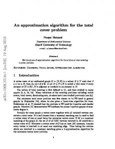
Figure 1: Visible Edge Decomposition

For points p, q ∈ P , Ray(p, q) denotes a ray starting from p which is collinear with line segment pq and is directed away from p. Each ray partitions the plane into two regions which we call left and right based on the ray’s direction. For each reflex vertex r and each edge e visible from r, we introduce two rays Ray(e1 (r), r) and Ray(e2 (r), r) in the interior Algorithm 1: Strategy RHL of P (see Fig 4.1(a)). We assume that these rays are line segments by restricting them to the interior of P . We write E(P ) for the partition of P formed by these 4 A New Decomposition line segments (Fig 4.1(b)). By a cell C ∈ E(P ) we First we define a decomposition which will be used mean a maximally connected region containing no as a building block for the partition decomposition. line segments. By the boundary B(C) of a cell we mean the set of line segments bounding it.

4.1

Visible edge decomposition

Let P denote a n-vertex simple polygon in the plane. An edge e of P is visible from a point p ∈ P if at least one interior point (i.e., a point except the end points) of e is visible from p. For a point p ∈ P, the edge skeleton E ∗ (p) is the subset of edges of P visible from p. Definition 4 A visible edge cell C is a maximally connected subset of P such that the edge skeletons E ∗ (p) = E ∗ (q) for any two points p, q contained in C. A visible edge decomposition is a partition of P into visible edge cells.

Lemma 3 E(P ) satisfies the following: (i) The cells of E(P ) are convex polygonal regions in the interior of P , and (ii) E ∗ (p) = E ∗ (q) for every two points p and q contained in a cell C ∈ E(P ). Proof: It is obvious that cells of E(P ) will be simple polygons. Let C be a cell with non-convex boundary. Let r be a reflex vertex on B(C). Clearly r cannot lie in the interior of P , as otherwise the two rays intersecting at r will further divide C. On the other hand, if r lies on P then r must be a vertex of P . But then the rays formed by the two edges of P adjacent to r

will divide C. Hence B(C) must be polygonal and convex. For the second part, take two points p, q contained in C such that E ∗ (p) 6= E ∗ (q). Let e be an edge in E ∗ (p) but not in E ∗ (q). Since B(C) is convex, the line segment l joining p and q is also contained in C. Let x be a point on pq such that e(x) reduces to a single point (such a point must exist). Let v1 and v2 be the vertices of P touching the line segment xe(x) from left and right respectively. Let v1 be the vertex closer to x than v2 . Then v1 is a reflex vertex of P and e(v1 ) has e(x) as one of its end points. Therefore Ray(e(x), v1 ) ∈ P intersects pq at x and hence subdivides C (a contradiction). ¥

Figure 2: The subpartition D(P, H12 )

Pi and Pj to get a preTheorem 1 E(P ) is a visible edge decomposition of follows: we first superimpose S liminary partition P P of the coordinate plane. i j P . E(P ) can be computed in time polynomial in n 4 D(P, Hij ) is then formed by takingSthe visible edge and has cardinality O(n ). decompositions of each cell in Pi Pj . (Note that Proof: The first part follows from lemma 3. As we do not take the visible edge decomposition of the E(P ) contains at most two rays for every pair of region formed by the intersection of the exteriors of a reflex vertex and an edge, it has at most O(n2 ) Pi and Pj .) As stated earlier, a cell C of a partition rays. Since at most O(n4 ) regions can be formed is a maximally connected region containing no line by O(n2 ) lines, this is an upper bound on the cardi- segments and its boundary B(C) is the set of segnality of E(P ). The decomposition can be computed ments bounding it. in polynomial time using obvious algorithms. ¥ Lemma 4 Let C be a cell of D(P, Hij . Then exactly one of the following holds: (i) V (p+hi ) = V (p+hj ) 4.2 Visibility Partition Decomposition for all coordinates p ∈ C or, (ii) V (p + hi ) 6= V (p + h Let P be the map polygon and H = j ) for all coordinates p ∈ C. T {h1 , h2 , . . . , hk } the set of active hypotheses. Proof: If C = ext(Pi ) ext(Pj ), then V (p + hi ) = Definition 5 For a set of hypotheses H, a visibil- V (p + hj ) = φ and we are S done. For the other case, let C be the cell of P Pj containing C. Let 1 i ity partition cell C is a maximally connected subset of the coordinate plane such that the visibility parti- S ⊂ B(C1 ) be the subset of edges of C1 visible from tions H(p) = H(q) for any two points p, q contained every point in C (recall that C is a cell of the visible in C. A visibility partition decomposition is a parti- edge decomposition E(C1 )). If an edge e ∈ S betion of the coordinate plane into visibility partition longs to just Pi , then V (p + hi ) 6= V (p + hj ) for all coordinates p ∈ C. On the other hand, if all edges in cells. S belong to both Pi and Pj then a robot at coordinate Let Pi denote a copy of the map polygon P in the p will see the same visibility polygon irrespective of coordinate plane such that hypotheses hi coincides whether it was initially at hi or hj . ¥ with the origin 0. For each pair of distinct hypothe- Lemma 5 D(P, H) satisfies the following: ses Hij = {hi , hj } we write D(P, Hij ) for the vis- (i) The cells of D(P, H) are polygonal regions, and ibility partition decomposition with respect to Hij . (ii) H(p) = H(q) for every two coordinates p, q conThe visibility partition decomposition D(P, H) for tained in a cell C of D(P, H). H is then constructed by taking the union of all line segments in the partitions {D(P, Hij )|1 ≤ i < j ≤ Proof: Every cell C ∈ D(P, H) is equal to the ink}. The construction of D(P, Hij ) (see Fig 4.2) is as tersections of cells Cij ∈ D(P, Hij ) containing it.

Since Cij ’s are polygons, C will be a polygon itself. For the second part, assume two points p, q contained in C such that H(p) 6= H(q). Choose a pair of hypotheses (hm , hn ) such that they belong to the same class in H(p) but not in H(q). Then p, q ∈ Cmn ∈ D(P, Hmn ) are two points such that V (p+hm ) = V (p+hn ) but V (q+hm ) 6= V (q+hn ), thereby contradicting lemma 4 above. ¥

that the other endpoint of C is unspecified. For a curve C, |C| denotes its length.

Theorem 2 For a simple polygon P and set of hypotheses H = {h1 , h2 , . . . , hk }, the visibility partition decomposition D(P, H) can be computed in polynomial time and has cardinality O(k 4 n8 ).

Proof: Consider a robot moving along curve C and continuously observing its environment. If the robot hits the boundary of P at coordinate x ∈ C, it localizes to a set of size at most |Blocked(x)| ≤ 21 |H| (since x ∈ PH∗ ). If the observation V taken by the robot at coordinate p ∈ C is different from the majority observation V (p, M aj(p)), the robot halflocalizes to a subset of H\M aj(p) which has size at most 12 |H|. The only other possibility is that the robot reaches the other end point of C without hitting the polygon P or taking a non-majority observation. However T the set of active hypotheses in this case |H| = | x∈C M aj(x)| ≤ 12 |H| (since C is a halving curve) and hence the robot half-localizes. ¥

Proof: That D(P, H) is a visibility partition decomposition S follows from lemma 5. The cardinality of Pi Pj is O(n2 ) and therefore the cardinality of D(P, Hij ) is O(n4 ). Hence D(P, H) is formed by at most O(k 2 n4 ) lines and is of total cardinality O(k 4 n8 ). The algorithm for computing D(P, H) follows from its construction above. ¥

Definition 7 AThalving curve is a curve C(0, .) ∈ PH∗ such that | x∈C M aj(x)| ≤ 12 |H|. Lemma 6 Let C ∈ PH∗ be a halving curve. A robot can correctly eliminate at least d 12 |H|e hypotheses by tracing C.

Corollary 1 By ignoring an arbitrarily small positive cost, robot movement can be assumed to be piecewise linear with breakpoints at edges of Lemma 7 There exists a halving curve of length at D(P, H). most HALF-OPT(P ,H). Proof idea: For each edge e of D(P, H), the first time the robot hits e (at an endpoint or interior) it can visit the interior of each cell adjacent to the relative interior of e at arbitrarily small cost. New information is acquired only at these limited times. Hereafter we assume that when the robot is at point q it can acquire all information available within arbitrarily small neighborhoods of q.

5

Halving Curves

Notation M aj(p) denote the maximum size class of visibility partition H(p). Blocked(p) denotes the class C of H(p) with V (C) = φ. Definition 6 A coordinate p is called halftraversable iff |Blocked(p)| ≤ 21 |H|. PH∗ is the maximally connected subset of half-traversable coordinates containing the origin.

Proof: Let S be an optimal strategy for HALFLOCALIZE(P ,H). Imagine a robot guided by S which stops as soon as it half-localizes. Let C(0, pf ) be the maximum length path traced by the robot in the coordinate plane for any (initial) position in H. By definition |C| ≤ HALF-OPT(P ,H). Let Hx denote the set of active hypotheses when the robot reaches coordinate x ∈ C. For x ∈ C\pf , |Hx | > 1 2 |H| since otherwise the robot would have stopped at x itself. Therefore |Blocked(x)| = |H| − |Hx | ≤ 1 ∗ 2 |H| and hence C ∈ PH . T Finally we show that the set I = x∈C M aj(x) is of size at most 12 |H|. For this assume a robot initially located at some h ∈ I ⊂ H. Guided by S, the robot would have followed path C and observed Vx = V (x, M aj(x)) forTall x ∈ C (since I ⊂ M aj(x)). But then |I| = | x∈C G(x, Vx )| = |Hpf | ≤ 12 |H| and hence C satisfies the lemma. ¥

∗ Corollary 2 Let CP,H denote the minimum length ∗ Notation C(u, v) denotes a curve in the coordi- halving curve. Then tracing CP,H is an optimal nate plane with end points u and v. C(u, .) means strategy for HALF-LOCALIZE(P ,H).

6

Reference Point Set

We are aiming to extract a polynomial size set of points on which to solve a group Steiner problem. The piecewise linear curves defined by these points come within a constant factor of the optimal halving curves. Notation. uv denotes the straight line segment joining points u and v. As before, the boundary B(C) of a cell C ∈ D(P, H) is the set of line segments bounding it.S The closure Clos(C) of a cell C is defined as C B(C). The interior of a cell is the cell minus its boundary. A cell C ∈ PH∗ iff every coordinate S in C lies in PH∗ . L denotes the set of line segments C∈P ∗ B(C). V denotes the set of H end points of segments in L. A vertex is a coordinate v ∈ V . For a point v and line segment l, let π(v, l) denote the point closest to v on l. For a set of points X and set of line segments Y, π(X, Y ) denotes the set of points {π(p, l)|p ∈ X, l ∈ Y }. The reference S point set Q0P,H = S S {0} V π(V, L) π(π(V, L), L). The size of Q0P,H is at most O(|V ||L|2 ) and it can be computed in polynomial time. ∗ Definition 8 A curve C(0, T .) ∈ PH is said to cover a cell C1 ∈ D(P, H) if C Clos(C1 ) 6= φ. The cover of C, Cover(C), is the set of all cells C1 ∈ D(P, H) covered by C.

For a piecewise linear curve C(u, v), BP (C) denote the set of its break points. For two curves C1 (u, v) and C2 (v, w), C1 ⊕ C2 denotes the curve with end points u, w formed by concatenating C1 and C2 . For a set S of cells in PH∗ , L∗S ∈ PH∗ denotes the shortest curve C(0, .) with one end point at origin such that S ⊆ Cover(L∗S ). We write the two end points of L∗S as 0 and e. For a curve C, C[u, v] denotes the portion of C with end points u and v. (i)SL∗S

Lemma 8 is piecewise linear, and S (ii) BP (L∗S ) {0, e} ⊆ C∈S B(C). Proof Idea: Part (i) is trivial. For the second part, consider a break point b ∈ BP (L∗S ) in the interior of a cell C ∈ D(P, H). Let b1 , b2 ∈ C be points infinitesimally preceding and succeeding b on L∗S . Then the curve L∗S [0, b1 ] ⊕ b1 b2 ⊕ L∗S [b2 , e] is strictly

shorter than L∗S (by triangle inequality) and covers S (a contradiction). ¥ The anchor of a break point b ∈ L∗S is the line segment lb ∈ L containing it. If b is a vertex, we arbitrarily choose one of the line segments containing it as its anchor. A break point is called a reflection point if it lies in the interior of its anchor. Clearly, every break point of L∗S is either (i) a vertex v ∈ V or, (ii) a reflection point. Lemma 9 Let r− , r+ be break points (or end points) immediately preceding and succeeding a reflection point r ∈ L∗S . Then r− and r+ lie on the same side of the line containing its anchor lr . Further r− and r+ lie on opposite sides of the line perpendicular to lr at r. Proof: Suppose r− , r+ lie on opposite sides of lr . Let C1 , C2 ∈ D(P, H) be cells containing the portion of L∗S in the neighborhood of r. Choose points p ∈ r− r, q ∈ rr+ such that pr, rq lie in Clos(C1 ) and Clos(C2 ) respectively and pq intersects lr . Then the curve obtained by replacing pr ⊕ rq by pq covers S and is strictly shorter than L∗S (a contradiction). Hence r− , r+ lie on same side of lr . For the second part, suppose r− , r+ lie on same side of the line perpendicular to lr at r. Choose point r0 ∈ lr on the same side of r as r− , r+ . Let r1 , r2 be points where the line perpendicular to lr at r0 intersects r− r, rr+ respectively. By choosing r0 close enough we can ensure that r1 r, rr2 ∈ Clos(C). Then the the curve formed by replacing r1 r ⊕ rr2 by r1 r0 ⊕ r0 r2 covers S and is strictly shorter than L∗S (a contradiction). ¥ Lemma 10 (i) The anchor lr of a reflection point r ∈ L∗S intersects L∗S only at r. (ii) If end point e is not a vertex, its anchor le intersects L∗S only at e. Proof: Suppose lr also intersects L∗S at r0 . Let C1 , C2 ∈ D(P, H) be cells adjacent lr . By lemma 9, the portion of L∗S in the neighborhood of r lies completely in one of Clos(C1 ) or Clos(C2 ). Let r1 , r2 be points infinitesimally preceding and succeeding r on L∗S such that triangle 4r1 rr2 lies completely in Clos(C1 ). Then the curve L∗S [0, r1 ] ⊕ r1 r2 ⊕ L∗S [r2 , e] covers S (it covers C2 at r0 ) and is strictly shorter than L∗S (a contradiction). ¥

set ui+1 = ui , vi+1 = v 0 . Otherwise let v 00 ∈ vi v 0 , u0 ∈ ui v 00 \{ui } be points as promised in Lemma 11 above. Set ui+1 = u0 , vi+1 = v 00 . Let Ci (u, vi ) denote the curve C(u, b)⊕bu1 ⊕. . .⊕ ui−1 ui ⊕ ui vi (see Fig 6(b)). The following properties are easySto establish by induction: (i) BP (Ci ) ⊆ BP (Ci−1 ) V , (ii) Cover(Ci ) ⊇ Cover(Ci−1 ) and (iii) |Ci | ≤ |Ci−1 | + |vi−1 vi |. (Use lemma 11 and the triangle inequality). Since ui ∈ V \{u0 , u1 , . . . , ui−1 }, there exists a k ≤ |V | such that vj = v 0 for all j ≥ k. Complete the proof by showing that C 0 = Ck satisfies the lemma. ¥. Figure 3: Lemmas 11 and 12 Lemma 11 Let uv ∈ PH∗ be a line segment such that v lies in the interior of lv ∈ L. Let v 0 be some other point on lv . Then either: (i) uv 0 ∈ PH∗ and Cover(uv) ⊆ Cover(uv 0 ), or (ii) there exist points v 00 ∈ vv 0 , u0 ∈ uv 00 \{u} such that u0 ∈ V , uv 00 ∈ PH∗ and Cover(uv) ⊆ Cover(uv 00 ).

Lemma 13 Let C(u, v) ∈ PH∗ be a piecewise linear curve such that v lies in the interior of a line segment lv ∈ L. Then there exists a piecewise linear curve C 0 (u, v 0 ) ∈ PH∗ such that (i) v 0 ∈ lv . v 0 is either an end point of lv or C 0 is perpendicular to lv at v 0 . 0 (ii) Cover(C) ⊆ Cover(C S ), 0 (iii) BP (C) ⊆ BP (C ) V and (iv) |C 0 | ≤ |C|.

S Proof Idea: Let b ∈ BP (C) {u} be the point immediately preceding v. Define a sequence {(ui , vi , vi0 )|i ≥ 0} as follows: (i) u0 = b, v0 = v. Set v00 = π(v0 , lv ). (ii) If Cover(ui vi ) ⊆ Cover(ui vi0 ) and ui vi0 ∈ PH∗ , 0 set ui+1 = ui , vi+1 = vi0 , vi+1 = vi0 . Otherwise let 00 0 0 00 v ∈ vi vi , u ∈ ui v \{ui } be points as promised in 0 Lemma 11 above. Set ui+1 = u0 , vi+1 = v 00 , vi+1 = π(ui+1 , lv ). Lemma 12 Let C(u, v) ∈ PH∗ be a piecewise linear The rest of the proof is similar to lemma 12, showing curve such that v lies in the interior of a line segment that for some 0 ≤ k ≤ |V |, the curve Ck (u, vk ) = lv ∈ L. Let v 0 be some other point on lv . Then there C(u, b) ⊕ bu1 ⊕ . . . ⊕ ui−1 ui ⊕ ui vi works. ¥ exists a piecewise linear curve C 0 (u, v 0 ) ∈ PH∗ such Lemma 14 Let r be a reflection point of L∗S and let that 0 ), r− and r+ be break points immediately preceding (i) cover(C) ⊆ Cover(C S and it. Then there exists a point r0 ∈ (ii) BP (C 0 ) ⊆ BP (C) V and, T succeeding 0 lr QP,H such that |rr0 | ≤ |r− r| + |rr+ |. (iii) |C 0 | ≤ |C| + |vv 0 |. Proof: Let vt , t ∈ [0, 1] denote the point tv + (1 − t)v 0 . Let t0 be the largest t such that Cover(uv) ⊆ Cover(uvt ) and uvt ∈ PH∗ . If t0 is 1, we satisfy part (i) of the lemma. Theorefore assume 0 ≤ t0 < 1. Take t0 > t0 arbitrarily close to t0 . By definition of t0 , there exists a cell C ⊆ Cover(uvt0 ) such that either C ∈ / Cover(uvt0 ) or uvt0 ∈ PH∗ . In either case it is easy to show that there exists a vertex u1 ∈ uvt0 \{u}. Take v 00 = vt0 , u0 = u1 (see Fig 6(a)). ¥

S Proof: Let b ∈ BP (C) {u} be the break point immediately preceding v. Define a sequence {(ui , vi )|i ≥ 0} as follows: (i) u0 = b, v0 = v. (ii) If Cover(ui vi ) ⊆ Cover(ui v 0 ) and ui v 0 ∈ PH∗ ,

Proof: Let lr denote the anchor of r. Let Π− , Π+ be lines perpendicular to Lr passing through r− , r+ respectively. Let H − , H + be half-spaces containing r bounded by Π− ,T Π+ respectively. H denotes the convex region H − H + .

r0 = 0 and rk = e as the two endpoints of L∗S and define r00 = r0 , rk0 = rk . Let Ci = L∗S [ri−1 , ri ], 0 < i ≤ k denote the subpath of L∗S from ri−1 to ri . Let Ci0 (ri−1 , ri0 ) be the piecewise linear curve promised by lemma 12 under the substitution 0 . Apply C = Ci , u = ri−1 , v = ri and v 0 = ri−1 0 , r 0 ). lemma 12 again to obtain Ci00 (ri−1 (Take i 0 0 0 C = Ci , u = ri , v = ri−1 and v 0 = ri−1 in this case). The following properties follow from lemma 12 itself: S S (i) B(Ci ) ⊆ B(Ci0 ) V ⊆ B(Ci00 ) V ⊆ V , (ii) Cover(Ci ) ⊆ Cover(Ci0 ) ⊆ Cover(Ci00 ) and 0 | ≤ |C | + |r 0 (iii) |Ci00 | ≤ |Ci0 | + |ri−1 ri−1 i i−1 ri−1 | + |ri ri0 |. Figure 4: Proof of lemma 14 Let v be a vertex in H. Clearly r0 = π(v, lr ) ∈ Q0P,H satisfies the lemma, since |rr0 | ≤ |r− r+ | ≤ |r− r| + |rr+ | (by triangle inequality). We complete the proof by finding a vertex v ∈ H. The only nontrivial case is shown in Fig 6: lr intersects π − and π + and both r− and r+ lie in the interior of their anchors lr− and lr+ respectively. Let v − , v + ∈ V denote the end points of lr− and lr+ lying in H − and H + respectively. Suppose on the contrary that v − ∈ H + and v + ∈ H − . Let q be the point where r− v − intersects Π+ . Since L is non-intersecting and lr− intersects L∗S only at r− (by lemma 10), q must lie on the portion of Π+ below (see Figure) r+ . Consider the quadrilateral Q formed by r, r− , q and r+ . Clearly Q ∈ H. Further since L is non-intersecting and lr+ intersects L∗S only at r− (lemma 10(ii) if r+ is an endpoint, else by lemma 10(i)), the segment r + e+ T + lies completely in Q. Therefore e ∈ H V (a contradiction). ¥ Theorem 3 (Geometric Approximation Theorem) There exists a piecewise linear curve LS (0, e0 ) ∈ PH∗ such that (i) S ⊆ Cover(L S ), S (ii) B(LS ) {0, e0 } ⊆ Q0P,H , and (iii) |LS | ≤ 5|L∗S |.

We show that LS = ⊕ki=1 Ci00 satisfies the theSk 00 orem. Since Cover(LS ) = i=1 Cover(Ci ) Sk ⊇ ⊇ Cover(L∗S ), i=1 Cover(C) LS covers S. S The set S of break points k 00 ) {r 0 , r 0 } (B(C ⊆ B(L ) ⊆ ( i i−1 i i=1 SS 0 0 0 0 0 V {r1 , r2 , . . . , rk−1 }. Since ri ∈ QP,H , 0 B(LS ) ⊆ QP,H . Finally the length of LS , k k P P 0 | + |r r 0 |) = |LS | = |Ci | ≤ (|Ci | + |ri−1 ri−1 i i i=1

|L∗S |

+ 2

i=1

k−1 P i=1

|ri ri0 |.

Since

ri0

was

cho-

sen according to lemma 14, this is at most k−1 P − |L∗S | + 2 (|ri ri | + |ri ri+ |) ≤ 5|L∗S |. Clearly the i=1

starting point origin lies in V . If the other endpoint rk = e lies in the interior of a line segment le , replace Ck00 by the curve promised by lemma 13 under the substitution C = Ck00 , u = rk−1 , v = e, lv = le . ¥

7 Group Steiner Problem and Main Result

Rooted 12 -Group Steiner Problem We are given a graph G = (V, E) with a cost function c : E →