John Paul Ekwaru and Stephen D. Walter
An Approximation for the Rank Adjacency Statistic for Spatial Clustering with Sparse Data
The rank adjacency statistic D provides a simple method to assess regional clustering. I t is dejned as the weighted average absolute diflerence in ranks of the data, taken over all possible pairs of adjacent regions. In this paper the usual normal approximation to the D statistic i s found to give inaccurate results fi the data are sparse and some regions have tied ranks. Adjusted formulae for the moments of D that allow for the existence of ties are derived. An example of analyses of sparse mortality data (with many regions having no death, and hence tied ranks) showed satisfactoy agreement between the adjusted formulae and the empirical distribution of the D statistic. We conclude that the D statistic, when used with adjusted moments, provides a valid approximate method to evaluate spatial clustering, even in sparse data situations. Maps are often used to convey pictorially the geographical variation of health data, such as incidence or death rates within a region, country or any geographical units (IARC 1989; Cislaghi et al. 1986; Clarke, Marrett, and Kreiger 1989; Pickle et al. 1996; WHO 1997; Le et al. 1995). Though visual assessment of these maps may reveal the presence of nonrandom patterns (existenceof clustering), statistical testing is required to confirm the pattern. Statistical measures such as the rank adjacency statistic D have been proposed for testing the nonrandomness of the observed patterns. The D statistic is defined as
This work was supported b International Clinical Epidemiology Network (INCLEN), Inc., and by NSERC Canada. The authors Lank Dr. Giuseppe Verlato (Universita Degli Studi Di Verona Instituto Di Igiene, Italy) for allowing them to use his data as an example.
John Paul Ekwaru is a lecturer in the Faculty of Medicine, Makerere University, Kampala. E-mail:
[email protected] Stephen D. Walter is a professor in the Department of Clinical Epidemiology and Biostatistics, McMaster University. E-mail:
[email protected] Geographical Analysis, Vol. 33, No. 1(January2001) The Ohio State University Revised version accepted: 4/18/00.
20 / Geographical Analysis where yi is the rank of the data value in region i; n is the number of regions in the study area; and w4 is a weight representing some function of distance, contact, or interaction between region i andj . The choice of weights depends on the study at hand and can be symmetric(w..= wji for all i,j) or asymmetric (wY# w . for ~ some ij).The simplest symmetricweighing option is a set of binary weights dedned as wq = 1 if regions i and j are adjacent, and 0 otherwise. Other reasonable symmetric weighting options include the inverse of the distance between the major population centers of regions i andj ; and the inverse of the number of boundaries shared between regions i and j . If the variable under study is migration or some other variable related to it, one might define asymmetric weights using directional migration value between regions i andj . Spatial clustering (that is, positive spatial autocorrelation) in the data will be reflected by a tendency for adjacent regions to have similar data ranks, so that the value of D will tend to be smaller. The D statistic was first proposed for summarizing cancer data in Scotland (IARC 1985) but it was only its expected value that was known analytdly. A test for its statistical significance could only be done by simulation, under the null hypothesis that the data values are randomly distributed across regions. The simulation process is computationally intensive, and a new set of simulations is required for each set of regions considered. The expected value of D is E(D) = (n+1)/3.
(2)
Walter derived an approximation for the variance of D, leading to an approximate significance test based on a standardized normal z ratio; the approximation proved very accurate in practical applications (Walter 1994), thus eliminating the previous need for simulation. The approximate variance derived by Walter is given by Var(D) = [(1/18)(n+l)(n-2)&$'- (1/9)XXr+,WrwsI/(X2Ur)2
(3)
where wr denotes a typical weight between a pair of regions. The above moments (2) and (3) of D are based on an assumption that each region in the study area has a unique rank, that is, no ties occur. If ties do occur, however, the sample space and the entire distribution of D is affected, and the approximate test based on moments (2) and (3) may be inaccurate. Ties are particularly likely if one is studying a rare event or if the regions have small populations, so that two or more regions have no observed cases, and hence have rates that are tied at zero. This occurred in the example discussed below. We shall refer to the above moments of D (mean and variance) calculated as previously, without allowing for possibility of ties, as unadjusted moments. EXAMPLE
During the period 1987-1991 deaths from cervical cancer occurred in only eighteen out of thirty-five social-heath units in Veneto region of Italy. Figure 1 shows the distribution of cervical cancer standardized mortality rates (SMR) in the region. The figures in parentheses are the number of units in each respective SMR interval. The numbers of cervical cancer deaths per unit ranged from 0 to 5 deaths, with eighteen social-healthunits having had no death, ten having had only a single death; one had 2 deaths, three regions had 3, two regions had 4, and one region had 5 deaths. Using binary weights as defined earlier, there were substantial differences between the unadjusted moments of the D statistic (obtained using the normal approximate
John Paul Ekwaru and Stephen D. Walter / 21
S M R 2307 - 2.614 (n=3) SMR: 1.861 - 2.141 (n=4) SMR: 1.624 - 1.697 (n=3)
SMR: 1.252 - 1.452 (n=4) SMR: 0.932 - 1.055 ( ~ 3 ) SMR: 0.000
(n=18)
FIG.1. Distribution of Standardized Mortality Rates (SMR) for Cervical Cancer among 15-to-54-YearOlds in the Veneto Region of Italy, 1987-1991
formulae), and the results obtained from the simulated distribution (see Table 1).Significance tests based on these two choices would give radically different conclusions. The unadjusted formulae give results that are obviously inaccurate, presumably because of the sparse data and the tied ranks. However, the distribution of D still appears to be approximately normal (Figure 2) even in this case, although there is moderate negative skewness of -0.344.This suggests that a z ratio test might be carried out even with sparse data, as long as adjusted formulae for the mean and variance can be determined. METHOD
We denote by m the number of regions with distinct ranks, and hence assume that
(n-m) regions are tied with zero events. For these regions we assume an average rank 0 = (n + m + l)/2. Though it is possible in general to have ties at nonzero values, this is very unlikely in practice when dealing with rates. TABLE 1 Test for Clusteringin Cervical cancer mortality in Veneto region 1987-91
Expected value: E ( D ) Variance: Var(D) P value for observed D=9.4312
Simulated Distribution
Normal Approximation
10.363 0.747 p =0.1389
12.000 0.715 p=0.0012
22 / Geographical Analysis 2400
4
1600
6
8 P
Fr,
000
0
6.3
6.8
7.3
7.0
8.3
8.8
9.3
9.8
10.3 10.8 11.3 11.8 12.3 12.8 13.3
Value ofthe D statistic. FIG.2. Simulated Null Distribution of the D Statistic
We now consider the mean and variance of D, under the null hypothesis that the ranks are randomly distributed in the regions, while allowing for ties. To simplify notation, we henceforth denote the typical value of d y (the absolute rank difference between region i andj) as d,. Then from the definition of the D statistic(1 )
E(D) = x & w q E ( d q ) / x q w y . Noting that E(dq)will be constant for any choice of i andj, we see that E(D) = E(dy), or E(D) = E(d,). To obtain an analytic expression for E(d,) we consider painvise differences for all the possible combinations of region ranks. We have two subsets of regions: set I consisting of regions with distinct ranks 1, ...m, and set 11consisting of regions with tied average rank u. Each possible air of regions would then be one of the three types as follows: (a) Both regions having distinct rates, that is, from set I. In this group the differencej (j=l,..., rn-1) occurs (m-j) times. (b) A region with a distinct rank paired with a region with a tied rank, that is, one member from set I and the other from set 11. If i is the distinct rank and u is the tied rank, then the difference u - i (i=l, ...,m) occurs n-m times. (c) Both regions having tied ranks, that is, from set 11. In this group, the difference 0 occurs (n-m)(n-m-1)/2 times. Since the total number of regions is n, we have a total of n(n-1)/2 possible pairs.
John Paul Ekwaru and Stephen D. Walter / 23 Hence summing over all possible differences of pairs, and after some simplification, we have that the adjusted mean of D is
"
E*(D)= E'(d) = -
n(n-1)
-
m
C ( m - j ) j + C (n-m)(u-j) + O j=l
j=l
m [3n2-3nm+m2-1]. 3n(n- 1 )
1
;
(4)
We will first obtain the adjusted value E"(d,")in a manner similar to that used to obtain E'(d,). We sum the squares of all the possible painvise differences as E"(d:) = -
m
1
C (m-j)j2 + C (n-m)(u-j)2 + o j=l
which after simplification gives E'(d:)=-
m [3n2-3mn+m - 13 6(n-1)
Hence,
- 3n2m[(n-l)(m2+3n-3nm-1)-6m(n-m)2]-(~4-~2)(m2+6~-6~~-1)
18n' (TI- 1)'
. (7)
To derive the adjusted covariance Cov'(d,, d,),+, we first calculate E(d,,d,),+ by considering all possible pairs of differences: (a) For difference pairs involving regions all in set I, the product of differences kj occurs (m-k)(m-j) times, i f j < k andj, k = 1,2....m-1; whenj=k, the product of differences kj = k 2 ( k = 1 , 2...m-2) occurs (m-k)(m-k-1)/2 times. (b) In pairs of differences involving one pair entirely from set I and one pair containing one region each from sets I and 11: the difference product ( u - i ) (i =1,2,....,rn;j= 1,2,....,(m- 1 ) ) occurs (n-m)(m-j) times; (c) In pairs of differences where each pair involves one member from set I and one member from set 11, the product ( u - i ) ( u - j ) occurs (n-m)' times when i