a minimum cardinality guarding set, but in this setting we must guard a simple .... segment hit; we add the edge (v, λ(y)) to a set E1 if v and λ(y) are of opposite.
An Approximation Scheme for Terrain Guarding Matt Gibson, Gaurav Kanade, Erik Krohn, and Kasturi Varadarajan⋆ Department of Computer Science University of Iowa Iowa City, IA 52242-1419, USA {mrgibson,gkanade,eakrohn,kvaradar}@cs.uiowa.edu
Abstract. We obtain a polynomial time approximation scheme for the terrain guarding problem improving upon several recent constant factor approximations. Our algorithm is a local search algorithm inspired by the recent results of Chan and Har-Peled [2] and Mustafa and Ray [15]. Our key contribution is to show the existence of a planar graph that appropriately relates the local and global optimum.
1
Introduction
A 1.5D terrain is a polygonal chain in the plane that is x-monotone, that is, any vertical line intersects the chain at most once. A terrain T consists of a set of m vertices {v1 , v2 , . . . , vm }. The vertices are ordered in increasing order with respect to their x-coordinates. There is an edge connecting vi with vi+1 for all i = 1, 2, . . . , m − 1. For any two points a, b ∈ T , we say that a sees b if the line segment ab lies entirely above or on the terrain. In this paper, we consider the discrete terrain guarding problem in which we are given a terrain T and finite sets X, G ⊆ T . For a set G′ ⊆ G, we say that G′ covers/sees/guards X if every point in X can be seen by at least one point in G′ . The goal of the problem is to find a minimum cardinality subset of G that covers X. The motivation for guarding terrains comes from placing street lights or security sensors along roads, as well as constructing line-of-sight networks for radio broadcasting and other communication networks [1]. A closely related problem is the art gallery problem. Again the goal is to find a minimum cardinality guarding set, but in this setting we must guard a simple polygon. The basic version of this problem, vertex guarding, requires guards to be placed at the vertices of the polygon. Another version, point guarding, allows guards to be placed anywhere inside the polygon. The art gallery problem was shown to be NP-complete by Lee and Lin [14] and was later shown to be APX-hard by Eidenbenz [7]. This means that there is an ǫ > 0 such that no polynomial time algorithm can compute a guarding set whose cardinality is within a (1 + ǫ) factor of the cardinality of an optimal guarding set, unless P = NP. Ghosh gives an O(log n)-approximation algorithm ⋆
Partially supported by NSF CAREER award CCR 0237431.
2
Gibson, Kanade, Krohn, Varadarajan
for vertex guarding an n-vertex simple polygon [11]. The point guarding problem seems to be much more difficult as not as much is known about it [5]. A constant factor approximation is given by Nilsson for the special case of the problem when the polygon is x-monotone [16]. Based on his result, Nilsson gives an O(OP T 2 )approximation algorithm for rectilinear polygons. Previous Work on Terrain Guarding. Chen et al. [3] claimed that terrain guarding is NP-hard, but the proof was never completed formally [12]. Most of the past research has gone into developing approximation algorithms. The first constant factor approximation was a combinatorial algorithm given by Ben-Moshe et al. [1]. Clarkson and Varadarajan [4] also give a constant factor approximation based on rounding a linear programming relaxation. King gave a simple combinatorial 4-approximation which was later determined to actually be a 5approximation [12]. Recently, Elbassioni et al. [8] gave a 4-approximation that also works for the weighted case. All of the approximation algorithms use the following “order claim”: Claim. Let a, b, c, d be four points on the terrain in increasing order according to x-coordinate. If a sees c and b sees d then a sees d. Natural attempts at constructing NP-hardness reductions for the terrain guarding problem do not work because of the order claim. Recently Krohn and King [13] were able to get around the order claim and prove NP-hardness. Our Contribution. We give a polynomial time algorithm that returns a guard cover whose cardinality is at most (1+ǫ)·OP T for any ǫ > 0. Here, OP T denotes the cardinality of an optimal guard cover. Thus we obtain the first PTAS for the problem improving upon several recent constant factor approximations. Given the hardness result [13], this settles the computational complexity of the problem. The inspiration for our work comes from the recent results of Chan and HarPeled [2] and Mustafa and Ray [15]. Chan and Har-Peled show that a local search algorithm actually yields a PTAS for the maximum independent set problem given a collection of disks. Unlike a previous PTAS for the problem [9], their analysis does not use packing arguments and thus also applies to “pseudo-disks”. Mustafa and Ray consider several geometric hitting set and set cover problems and describe local search algorithms that yield PTASs. For instance, in a rather surprising result they obtain a PTAS for the problem of covering a set of points by the smallest number of a given set of disks. Both papers use separator theorems for planar graphs. In particular, they show that there exists a planar graph that relates the locally optimal solution returned by the local search and the global optimal solution. The separator theorem is then used to show that the locally optimal solution is not too much worse than the global optimum. Our PTAS for the terrain guarding problem is also based on local search. Our key contribution is to show the existence of an appropriate planar graph even for the terrain guarding context. Having shown this, the rest of the analysis is very similar to that of Mustafa and Ray [15].
An Approximation Scheme for Terrain Guarding
2
3
Guarding Terrains via Local Search
Recall that our input is a polygonal terrain, a set X of points on the terrain that need to be guarded, a set G of possible guard locations, and a parameter 0 < ǫ < 1. For purposes of exposition, we will initially assume that X ∩ G = ∅. We later show how this assumption can be removed. We describe a polynomial time algorithm that returns a subset Q ⊆ G that sees X, so that |Q| is at most a factor (1 + ǫ) times the size of the smallest subset of G that sees X. Let n denote the input size – the number of vertices in the terrain, plus |G|, plus |X|. We say that a subset of G that sees X is b-locally optimal if one cannot obtain a smaller set of guards that sees X by deleting at most b guards from it and inserting at most b − 1 guards. Our algorithm simply returns a b-locally optimal solution for b = ǫα2 , where α is a suitably large constant, by performing local search. We start with some arbitrary Q ⊆ G that covers X. For every subset S ⊆ Q of size at most b, we see if there exists a subset T ⊆ G \ Q of size at most |S| − 1 such that (Q \ S) ∪ T guards X. If so, we set Q ← (Q \ S) ∪ T . Every such exchange decreases the size of �Q by at least one, and as such can happen at most n times. Since there are n O(b) . b subsets S to consider, the running time is bounded by n 2.1
Approximation Analysis
Let R′ denote the optimal cover for X, and B ′ the set of guards output by our local search algorithm on termination. We show that |B ′ \ R′ | ≤ (1 + ǫ)|R′ \ B ′ |, and thus |B ′ | ≤ (1 + ǫ)|R′ |. Let R ≡ R′ \ B ′ , B ≡ B ′ \ R′ , and abusing notation, let X denote the set after removing all points seen by R′ ∩ B ′ . So now both R and B cover X and we wish to show that |B| ≤ (1 + ǫ)|R|. We will refer to points in B as blue points and points in R as red points. The following lemma is our main contribution; it shows that the locality condition of Mustafa and Ray [15] is satisfied. Lemma 1. There exists a planar graph G = (V ≡ R ∪ B, E) with the property that for each x ∈ X, there is an edge (r, b) in G between guards r ∈ R and b ∈ B that both see x. Before giving the proof, we show how the lemma implies that |B| ≤ (1+ǫ)|R|; this is similar to [2, 15]. We need the following partition theorem on planar graphs due to Frederickson [10]. For U ⊆ V , let Γ (U ) denote the set of neighbors in G of vertices in U with U excluded. Let µ = |V |. Lemma 2. √ For any parameter 1 ≤ r ≤ µ, we can find a set S ⊆ V of size at V \ S into µ/r sets V1 , V2 , . . . , Vµ/r , satisfying most c1 µ/ r and a partition of √ (i) |Vi | ≤ c2 r, (ii) |Γ (Vi )| ≤ c3 r, and (iii) (Vi ∪ Γ (Vi )) ∩ Vj = ∅ for i 6= j. Here, c1 , c2 , and c3 are absolute positive constants. √Let us apply the lemma with r ≡ b/(c2 + c3 ). We have |Vi ∪ Γ (Vi )| ≤ c2 r + c3 r ≤ b. Thus, letting Ri = R ∩ Vi and Bi = B ∩ Vi , we must have |Bi | ≤
4
Gibson, Kanade, Krohn, Varadarajan
|Ri | + |Γ (Vi )|. For otherwise, the local search can replace Bi by Ri ∪ Γ (Vi ) and obtain a smaller set that still covers X (Lemma 1), a contradiction. Thus X X X µ |Γ (Vi )| ≤ |R| + c √ |Ri | + |Bi | ≤ |S| + |B| ≤ |S| + r i i i ≤ |R| + c′
|R| + |B| √ , b
where c and c′ are positive constants. With b a large enough constant times 1/ǫ2 , this implies that |B| ≤ (1 + ǫ)|R|. 2.2
Proof of Lemma 1
We begin with some notation. For points a and b on the terrain, we say a ≤ b to mean that the x-coordinate a.x of a is at most b.x. We use the notation of intervals that this implies – for instance, [a, b] denotes all points c on the terrain so that a ≤ c ≤ b. We now prove Lemma 1. Let us first construct the planar graph G. For each x ∈ X, let λ(x) denote the leftmost point that sees x among points in R ∪ B to the left of x, assuming such a point does exist. Similarly, let ρ(x) denote the rightmost point that sees x among points in R ∪ B to the right of x, assuming such a point does exist. Note that at least one of λ(x) or ρ(x) does exist. Let A1 denote the set of segments λ(x)x, for x ∈ X. Because of the order claim, these segments do not cross. For each v ∈ R ∪ B, shoot a vertical ray up from v; if this ray hits some segment in A1 , let λ(y)y denote the first such segment hit; we add the edge (v, λ(y)) to a set E1 if v and λ(y) are of opposite colors. Now, the edges in A1 ∪ E1 can be embedded above the terrain in a noncrossing way. To see this, let A1 be embedded as the original straight line segments. To embed an edge of the form (v, λ(y)) ∈ E1 as above, we travel straight up from v till we hit λ(y)y, and then slide along the segment λ(y)y to reach λ(y). See Figure 1. A more formal argument that A1 ∪ E1 can be so embedded is given in the appendix. Let A2 denote the set of segments xρ(x), for x ∈ X. Again, these segments do not cross. For each v ∈ R ∪ B, shoot a vertical ray up from v; if this ray hits some segment in A2 , let yρ(y) denote the first such segment hit; we add the edge (v, ρ(y)) to a set E2 if v and ρ(y) are of opposite colors. The edges in A2 ∪ E2 can also be embedded above the terrain in a noncrossing way. We “flip” the embedding of A1 ∪ E1 to obtain a non-crossing embedding below the terrain; see Figure 2. This gives us a planar embedding of A1 ∪ E1 ∪ A2 ∪ E2 . Finally, for each x ∈ X, we add the edge (λ(x), ρ(x)) to a set E3 if λ(x) and ρ(x) are of opposite colors. Our graph G consists of the edge set E1 ∪E2 ∪E3 . This is a planar graph; just embed E1 and E2 as above, and for each (λ(x), ρ(x)) ∈ E3 , embed it using the embedding of the segments λ(x)x and xρ(x).
An Approximation Scheme for Terrain Guarding
5
11 00 00 11 v0 1 0 0 v1 1
0 1
0 x1
1′′ 0 0 1 x
v2 0 1
1 v0 3
1111 00 00 00 11 ′ v4 11 00 x
Fig. 1. The embedding of A1 ∪E1 , with X = {x, x′ , x′′ }, and R∪B = {v0 , v1 , v2 , v3 , v4 }. Segments in A1 are shown in dashed lines, and the edges in E1 are embedded as dashed curves with arrows. Note that v0 = λ(x) = λ(x′′ ), and v2 = λ(x′ ).
1 0
1 0
1 0 x
1 00 0 11
1 0 v4
1 0 ′ x
1 0 ′′
1 0
1 0
1 0 01
11 00
1 0
1 0
1 0
v0
v1
v2
v3
x
Fig. 2. A combinatorial embedding of A1 ∪ E1 from Figure 1, and flipping it so that A1 ∪ E1 is now embedded below the terrain. Note that only the edges in A1 ∪ E1 are being flipped to make room for A2 ∪ E2 ; the vertex set R ∪ B ∪ X retains its embedding.
6
Gibson, Kanade, Krohn, Varadarajan
Now we need to show that for each x ∈ X, there are points r ∈ R and b ∈ B that see x, and (r, b) ∈ E1 ∪ E2 ∪ E3 . Fix an x ∈ X. If λ(x) and ρ(x) are of opposite colors, then (λ(x), ρ(x)) ∈ E3 , and we are done. Otherwise, it must be the case that there are red and blue points to the left of x that see x, or that there are red and blue points to the right of x that see x. Let us assume that the first case holds (there are red and blue points to the left of x that see x), and that λ(x) is red. The other situations are symmetric. Let b be the leftmost blue point that sees x; it must be that b ∈ (λ(x), x). Thus the ray shot up from b hits λ(x)x; let λ(y)y be the first segment in A1 that it hits. See Figure 3. Because segments in A1 don’t cross, it must be that λ(y) ∈ [λ(x), b) and y ∈ (b, x). The order claim (applied to λ(y), b, y, and x) implies that λ(y) sees x. Now λ(y) cannot be blue, otherwise b is not the leftmost blue point that sees x. Thus λ(y) ∈ R, b ∈ B, both λ(y) and b see x and (b, λ(y)) ∈ E1 . This completes the proof.
λ(x) λ(y)
x y b
Fig. 3. Here, λ(y) sees y and b sees x. By the order claim, λ(y) sees x.
2.3
Relaxing the Disjointness Assumption
For ease of exposition, we have so far assumed that the set of possible guard locations has an empty intersection with the set of points to be guarded. We now relax that assumption. The algorithm remains unchanged, and we indicate how the analysis is modified. For each x ∈ X, the point λ(x) (resp. ρ(x)) denotes the leftmost (resp. rightmost) point that sees x among points in R ∪ B strictly to the left (resp. right) of x, assuming such a point does exist. With this understanding, the construction of the planar graph G proceeds with the sets A1 , E1 , A2 , and E2 defined exactly as above. There is a change in the construction of E3 . For each x ∈ X that is not in R ∪ B, we proceed as before and add the edge (λ(x), ρ(x)) to E3 if λ(x) and ρ(x) are of opposite colors. For x ∈ X that is also in R ∪ B, we add the edge (λ(x), x) to E3 if λ(x) exists and λ(x) and x are of opposite colors; we also add the edge (x, ρ(x)) to E3 if ρ(x) exists and ρ(x) and x are of opposite colors.
An Approximation Scheme for Terrain Guarding
7
This completes the construction of the graph, which is readily seen to be planar. To show Lemma 1, we need to argue that for each x ∈ X, there are points r ∈ R and b ∈ B that see x, and (r, b) ∈ E1 ∪ E2 ∪ E3 . If x 6∈ R ∪ B then the argument is exactly as before. Without loss of generality, assume that x ∈ R. Since B sees X, there must be a point in B that sees x. Assume that such a blue point lies to the left of x. The other case is symmetric. In this case, it must be that λ(x) exists. If λ(x) ∈ B, then we are done since we added (λ(x), x) to E3 . Therefore assume that λ(x) ∈ R. Let b be the leftmost blue point that sees x. Now we can use the reasoning in the last paragraph of the previous section to show that there is an edge (b, u) ∈ E1 such that both b and u see x, b is blue, and u is red.
3
Conclusions
We have shown that the discrete terrain guarding problem admits a polynomialtime approximation scheme. We can also obtain a PTAS in the scenario where the possible guard locations are from a finite set, and we want to see the entire terrain – this problem is readily reduced to discrete terrain guarding. In the continuous terrain guarding problem, guards are allowed to be located anywhere on the terrain. The local search can be seen to work even here, and we can show that a single iteration of the local search can be implemented in polynomial time along the lines of Section 4 of [6]. There is one issue that remains, however, and this is to bound the number of bits needed to represent the guards maintained by the local search. We are currently investigating how this can be handled. Acknowledgements. We thank the anonymous reviewers for useful feedback.
References 1. Boaz Ben-Moshe, Matthew J. Katz, and Joseph S. B. Mitchell. A constant-factor approximation algorithm for optimal terrain guarding. In SODA, pages 515–524, 2005. 2. Timothy Chan and Sariel Har-Peled. Approximation algorithms for maximum independent set of pseudo-disks. In Symposium on Computational Geometry, 2009. To Appear. 3. Danny Z. Chen, Vladimir Estivill-Castro, and Jorge Urrutia. Optimal guarding of polygons and monotone chains (extended abstract), 1996. 4. Kenneth L. Clarkson and Kasturi Varadarajan. Improved approximation algorithms for geometric set cover. In SCG ’05: Proceedings of the twenty-first annual symposium on Computational geometry, pages 135–141, New York, NY, USA, 2005. ACM. 5. Ajay Deshpande, Taejung Kim, Erik D. Demaine, and Sanjay E. Sarma. A pseudopolynomial time o(log 2 n)-approximation algorithm for art gallery problems. In Proceedings of the 10th Workshop on Algorithms and Data Structures (WADS 2007), volume 4619 of Lecture Notes in Computer Science, pages 163–174, Halifax, Nova Scotia, Canada, August 15–17 2007.
8
Gibson, Kanade, Krohn, Varadarajan
6. Alon Efrat and Sariel Har-Peled. Guarding galleries and terrains. Information Processing Letters, 100(6):238 – 245, 2006. 7. Stephan Eidenbenz. Inapproximability results for guarding polygons without holes. In Lecture Notes in Computer Science, pages 427–436. Springer, 1998. 8. Khaled Elbassioni, Erik Krohn, Domagoj Matijevic, Julian Mestre, and Domagoj Severdija. Improved approximations for guarding 1.5-dimensional terrains. In Susanne Albers and Jean-Yves Marion, editors, 26th International Symposium on Theoretical Aspects of Computer Science (STACS 2009), Dagstuhl, Germany, 2009. Schloss Dagstuhl - Leibniz-Zentrum fuer Informatik, Germany. 9. Thomas Erlebach, Klaus Jansen, and Eike Seidel. Polynomial-time approximation schemes for geometric intersection graphs. SIAM Journal on Computing, 34(6):1302–1323, 2005. 10. Greg N. Frederickson. Fast algorithms for shortest paths in planar graphs, with applications. SIAM J. Comput., 16(6):1004–1022, 1987. 11. S. Ghosh. Approximation algorithms for art gallery problems, Proc. Canadian Information Processing Society Congress, 1987. 12. James King. A 4-approximation algorithm for guarding 1.5-dimensional terrains. In Proc. of the 7th Latin American Symposium on Theoretical Informatics (LATIN’06), pages 629–640, Valdivia, Chile, 2006. 13. Erik Krohn and James King. The complexity of guarding terrains, Manuscript, 2009. 14. D. Lee and A. Lin. Computational complexity of art gallery problems. Information Theory, IEEE Transactions on, 32(2):276–282, Mar 1986. 15. Nabil H. Mustafa and Saurabh Ray. Ptas for geometric hitting set problems via local search. In Symposium on Computational Geometry, 2009. To Appear. 16. Bengt J. Nilsson. Approximate guarding of monotone and rectilinear polygons. In ICALP, pages 1362–1373, 2005.
A
Appendix
We present here a more formal argument for a piece of Lemma 1 that shows that the graph (X ∪ R ∪ B, A1 ∪ E1 ) has a planar embedding with X ∪ R ∪ B on a horizontal line and A1 ∪ E1 drawn above the line. We now think of A1 as a set of combinatorial edges rather than as line segments. Let us say that two edges in A1 ∪ E1 cross if all four end points are distinct, and can be ordered as a < b < c < d with the edges being (a, c) and (b, d). Notice that crossing in this sense is determined entirely by the ordering of the endpoints, and makes no reference to a drawing of the edges. We first argue that no two edges in A1 ∪ E1 cross. 1. Let (λ(x), x) and (λ(y), y) be any two edges in A1 . They do not cross, for if λ(x) < λ(y) < x < y, then by the order claim, y sees λ(x), contradicting the definition of λ(y). 2. We argue that an edge in A1 and an edge in E1 do not cross. Let us recall how edges in E1 are defined. Let us say that an edge (λ(x), x) is above v ∈ R ∪ B if λ(x) < v < x. We look at all edges in A1 that are above v, and if this set is non-empty we find the “innermost” such edge (λ(y), y). We add the
An Approximation Scheme for Terrain Guarding
9
edge (λ(y), v) to E1 if λ(y) and v are of opposite colors. Let us say that (λ(y), y) ∈ A1 defines (λ(y), v) in this case. Now suppose (λ(y), v) crosses some (λ(x), x) ∈ A1 . Now if λ(x) < λ(y) < x < v, then (λ(x), x) and (λ(y), y) cross, a contradiction. On the other hand, if λ(y) < λ(x) < v < x, there are two cases: either x ≤ y, in which case the contradiction is that (λ(y), y) is not the innermost edge in A1 that is above v; or x > y, in which case the contradiction is that (λ(y), y) and (λ(x), x), which are both edges in A1 , cross. 3. We now show that no two edges in E1 cross. Consider two such edges (λ(y1 ), v1 ) and (λ(y2 ), v2 ), defined by (λ(y1 ), y1 ) and (λ(y2 ), y2 ) respectively. These edges do not cross, for if λ(y1 ) < λ(y2 ) < v1 < v2 , then (λ(y1 ), v1 ) crosses (λ(y2 ), y2 ), which contradicts the fact that an edge in E1 and an edge in A1 do not cross. Thus, no two edges in A1 ∪ E1 cross. From this, it follows that the required embedding exists. For instance, embed the vertices X ∪ B ∪ R as distinct points in the correct order on the lower half of the unit circle, and draw the edges in A1 ∪ E1 as straight line segments. Using convexity arguments, this can be seen to be a planar embedding. Now we “bend” the lower half of the unit circle into a horizontal segment, allowing the drawing of edges in A1 ∪ E1 to now become curved.