1810
JOURNAL OF ATMOSPHERIC AND OCEANIC TECHNOLOGY
VOLUME 18
An Areal Rainfall Estimator Using Differential Propagation Phase: Evaluation Using a C-Band Radar and a Dense Gauge Network in the Tropics V. N. BRINGI, GWO-JONG HUANG,
AND
V. CHANDRASEKAR
Department of Electrical and Computer Engineering, Colorado State University, Fort Collins, Colorado
T. D. KEENAN Bureau of Meteorology Research Center, Melbourne, Victoria, Australia (Manuscript received 20 December 2000, in final form 13 April 2001) ABSTRACT An areal rainfall estimator based on differential propagation phase is proposed and evaluated using the Bureau of Meteorology Research Centre (BMRC) C-POL radar and a dense gauge network located near Darwin, Northern Territory, Australia. Twelve storm events during the summer rainy season (December 1998–March 1999) are analyzed and radar–gauge comparisons are evaluated in terms of normalized error and normalized bias. The areal rainfall algorithm proposed herein results in normalized error of 14% and normalized bias of 5.6% for storm total accumulation over an area of around 100 km 2 . Both radar measurement error and gauge sampling error are minimized substantially in the areal accumulation comparisons. The high accuracy of the radar-based method appears to validate the physical assumptions about the rain model used in the algorithm, primarily a gamma form of the drop size distribution model, an axis ratio model that accounts for transverse oscillations for D # 4 mm and equilibrium shapes for D . 4 mm, and a Gaussian canting angle distribution model with zero mean and standard deviation 108. These assumptions appear to be valid for tropical rainfall.
1. Introduction The differential propagation phase (Fdp ) between horizontal and vertical polarization due to rain at microwave frequencies is now well known to be an important radar measurement, in particular for estimating rain amounts (Seliga and Bringi 1978; Sachidananda and Zrnic´ 1987). In particular, Fdp-based methods offer many practical advantages over power-based methods, for example, immune to radar system gain variations, attenuation effects, beam blockage (Zrnic´ and Ryzhkov 1996). The Fdp field can be naturally expressed in polar coordinates (r, u), where r is the radar range and u is the azimuth angle, when the radar scans the rain area at low elevation angle in the usual plan position indicator (PPI) mode. It was recognized by Raghavan and Chandrasekar (1994) in the context of area–time integral methods, that the azimuthal sweep of Fdp across the rain area can be viewed as an areal integration of the instantaneous rain-rate field. Thus, to calculate the mean areal rain rate (R ), it is not necessary to know the specific differential phase [Kdp 5 (1/2)dFdp /dr], which is a ‘‘noisy’’ measure and involves substantial smoothing of Corresponding author address: Prof. V. N. Bringi, Department of Electrical and Computer Engineering, Colorado State University, Fort Collins, CO 80523-1373. E-mail:
[email protected]
q 2001 American Meteorological Society
the Fdp field (e.g., Hubbert and Bringi 1995). In particular, large gradients of reflectivity can cause the estimated Kdp to be biased (Gorgucci et al. 1999). The areal rainfall method using Fdp for estimating R does not involve the prior estimation of Kdp . Therefore, this method preserves all the practical advantages of the Fdp measurement and avoids the major disadvantage of computing Kdp , the only trade-off being that an areal estimate of R is available. Another advantage of the areal Fdp method is related to validation using a dense network of gauges. It is well known that the usual method of comparing radar rain rates over single gauges is fraught with large uncertainty, and that a significant portion of the variance may be due to gauge sampling error, that is, point gauge estimates cannot accurately represent rainfall over typical radar pixel sizes (e.g., 2 km 3 2 km), see, for example, Anagnostou et al. (1999). However, the gauge sampling error can be substantially reduced if a dense network of gauges is used, and, hence, the mean areal rainfall from the network can be used to validate areal Fdp algorithms more robustly as compared to individual radar–gauge comparisons. It follows that the physical basis of areal Fdp algorithms can be evaluated by intercomparison with a dense gauge network. In particular, since a parametric form is often used to convert from areal Fdp to R , the parameterization errors (arising from
NOVEMBER 2001
1811
BRINGI ET AL.
drop size distribution fluctuations and choice of drop shape models) are likely to dominate the variance between the radar and gauge comparisons. In this paper, an areal Fdp estimator is proposed that is philosophically somewhat different from Ryzhkov et al. (2000). In order to estimate the mean areal rain rate from the azimuthal sweep of Fdp , a linear R–Kdp relation is assumed to be valid locally (R 5 cKdp ). However, from physical considerations, the relation between R and Kdp at long wavelengths is somewhat nonlinear (Sachidananda and Zrnic´ 1987). This nonlinearity is accounted for by adopting a piecewise linear fit to specify the R–Kdp relation. On the other hand, the areal Fdp estimator of Ryzhkov et al. (2000) preserves the nonlinear form for R–Kdp , but assumes that Kdp is constant along radials intercepting the area of interest. Model simulations are used to compare these two estimators using various range profiles of Kdp . Validation of the areal Fdp algorithm developed in this paper is based on comparison with a dense gauge network located near Darwin, Northern Territory, Australia. The Bureau of Meteorology Research Center (BMRC) C-POL radar (frequency near 5.5 GHz) located near Darwin provided the Fdp data (Keenan et al. 1998). Twelve storm events are analyzed from the summer rainy season (December 1998–March 1999), which included a variety of rainfall types. This paper is organized as follows. Background material is provided in section 2 on the two areal rainfall estimators, and model simulations are used to understand the differences between these two estimators. Ra-
AR 5
c 2
E5
dar data processing details are dealt with in section 3, together with a brief discussion of the radar–gauge comparison methodology. In section 4 the result of the radar–gauge comparisons is discussed, while section 5 provides a short summary and discussion of results. 2. Background The areal rainfall AR can be defined as AR 5
EE r2
AR 5
r1
(1)
u2
R(r, u )r dr du.
(2)
u1
If a linear relationship between R and Kdp is assumed of the form R 5 cKdp , and using Kdp 5 ½(d/dr)(Fdp ), (2) can be expressed as AR 5 5
c 2 c 2
E E E E u2
r2
du
u1
r1
u2
(3)
r dFdp (r, u).
(4)
r2
du
u1
d F (r, u )r dr dr dp
r1
Integrating by parts results in
[r2 Fdp (r2 , u ) 2 r1Fdp (r1, u )] 2
In the above formula, for a given beam with constant u, AR depends on its boundary values at r1 and r 2 as well as on the area under the Fdp versus range profile. As the azimuthal angle changes from u1 to u 2 , an areal sweep of Fdp over the rain region occurs naturally performing a spatial integration of the rainfall. Thus, it is not necessary to estimate Kdp (r), which is a noisy field because it is obtained as one-half of the range derivative of Fdp (r). On the other hand, the Fdp (r) is easily smoothed in range (Hubbert and Bringi 1995) and an accurate estimate of AR is readily available. However, some error is introduced since the R–Kdp relation is somewhat nonlinear, that is, at long wavelengths, R 5 aK bdp where b ø 0.85 (Sachidananda and Zrnic´ 1987; Chandrasekar et al. 1990). To reduce this error, a piecewise linear fit is proposed as illustrated in Fig. 1. The data points are based on 2-min averaged drop size distributions (dsd) from a disdrometer (Joss and Waldvogel
R(x, y) dx dy,
where R(x, y) is the instantaneous rain-rate field. The mean areal rain rate R is defined as AR divided by the corresponding area. The use of polar coordinates is suitable for low-elevation angle radar data acquired in the conventional PPI scan mode. If r is the range and u is the azimuth angle, the areal rainfall in polar coordinates is
u2
u1
EE
E
r2
r1
6
Fdp (r, u ) dr du.
(5)
1967) located in Darwin, Northern Territory, Australia (details are provided in the appendix). These data are representative of an entire rainy season in Darwin. The Kdp calculations are performed at a frequency of 5.5 GHz (C band) and assuming that raindrop axis ratios (for 1 # D # 4 mm) obey the relation given in Andsager et al. (1999), and for D , 1 or D . 4 mm the relation given in Beard and Chuang (1987). In addition, a Gaussian canting angle distribution is assumed with zero mean and standard deviation of 108. This model is believed to be applicable for tropical rainfall [see chapter 7 of Bringi and Chandrasekar (2001)]. The multiplicative coefficient c in (5) is selected from the piecewise fit based on the average Kdp value in the range interval r1 to r 2 for any given beam. The areal rainfall estimate based on (5) and the piecewise linear fit in Fig. 1 will be termed the Colorado State University (CSU) estimate. When AR in (5) is divided by the corresponding area, it will
1812
JOURNAL OF ATMOSPHERIC AND OCEANIC TECHNOLOGY
FIG. 1. Scattering simulations at C band based on measured drop size distributions from Darwin (each data point refers to a 2-min averaged dsd; see the appendix for details). Also, the piecewise linear fit is illustrated. A nonlinear fit to the data points results in R 5 32.4(Kdp ) 0.83 .
be termed the R csu algorithm or simply the CSU algorithm. The formula for AR proposed and evaluated by Ryzhkov et al. (2000), henceforth referred to as RZF, is based on a nonlinear relation R 5 aK bdp (here, a 5 32.4, b 5 0.83 from scattering simulations described above). It is assumed that Kdp (r, u) is constant for a given u. It follows that (2) can be simplified as
E E u2
AR rzf 5
r2
du
u1
b aK dp (r, u )r dr
r1
E
a 5 (r22 2 r12 ) 2
(6)
u2 b K dp (u ) du
(7)
VOLUME 18
FIG. 2. The idealized Kdp profiles used in the model simulations: (a) profiles marked 1–3, (b) Gaussian profiles marked 4–6.
2 r1 ) is small, then (9) becomes more exact, but the accuracy of the approximation depends not only on (r 2 2 r1 ) but also on how different the actual Kdp (r) profile is from being a constant. For both areal Fdp estimators, the measurement error is virtually negligible because of the areal integration and prior smoothing of the Fdp range profiles [see the appendix of Ryzhkov et al. (2000)]. To investigate the differences between (5) and (9), several model Kdp (r) profiles are chosen as illustrated in Figs. 2a,b and simulations are used (assuming u 5 constant) to compare ARcsu and ARrzf against the ‘‘exact’’ value using (2) with R 5 32.4K 0.83 dp . Figure 3 shows the percentage error in ARcsu and ARrzf versus the Kdp profile number (each number from 1 to 6 corresponds to a particular profile in Fig. 2). It is clear that ARcsu ,
u1
a 5 (r2 1 r1 )(r2 2 r1 ) 2 3
E
u2
du
u1
5
1
[
]
Fdp (r2 , u ) 2 Fdp (r1, u ) 2(r2 2 r1 )
b
(8)
2
a r2 1 r1 [2(r2 2 r1 )]12b 2 2 3
E
u2
[Fdp (r2 , u ) 2 Fdp (r1, u )] b du.
(9)
u1
When the above AR is divided by the corresponding area it will be termed the R rzf algorithm or simply the RZF algorithm. In this formula, only the boundary values of Fdp occur for each beam; thus it is simpler to implement as compared with (5). However, the rangeweighting, which is exact in (5), is constant in (9); that is, the range-weighting is constant at (r 2 1 r1 )/2. If (r 2
FIG. 3. The percentage error in areal rainfall (AR) using the CSU estimator [see (5)] and the RZF estimator [see (9)] vs the Kdp profile number (see Fig. 2).
NOVEMBER 2001
BRINGI ET AL.
1813
FIG. 4. Model Gaussian-shaped profile of Kdp used in simulations shown in Fig. 5.
FIG. 5. The percentage error in areal rainfall using the CSU estimator (ARcsu ) and the RZF estimator (ARrzf ) vs (r 2 2 r1 ). Note that r1 5 40 km (see Fig. 4), whereas r 2 in this figure is variable.
even with the piecewise linear fit, has small error (#10%) while ARrzf can have large error (e.g., profile 5), especially when the Kdp profile is asymmetrically located relative to the center (r1 1 r 2 )/2, with its peak value closer to r1 . Moreover, from the results of Fig. 3, the error in ARcsu appears to fluctuate from 210% to 110% depending on the shape of the Kdp profile whereas the error in ARrzf appears to be one-sided. In practice, this implies that the error in ARcsu should tend to balance out as the actual Kdp profiles will tend to vary more or less randomly in shape. To further illustrate the error caused by constant range-weighting in ARrzf , Fig. 4 shows an idealized Gaussian profile of Kdp centered near 50 km; note that r1 5 40 km is fixed whereas r 2 is allowed to vary from 60 to 100 km. Figure 5 shows the percentage error in ARcsu and ARrzf versus (r 2 2 r1 ). These idealized simulations show that the error in ARcsu is bounded to #10% whereas the error in ARrzf increases with (r 2 2 r1 ) and does not appear to be bounded. Note that these model simulations are based on a constant r1 . The error in ARrzf , in general, will depend on both (r 2 2 r1 ) as well as the mean range, (r 2 1 r1 )/2.
cedures were used to reject faulty gauge data (May et al. 1999). For each gauge, 1-min rain rates (Rg) were available as a time series. Raindrop size distribution data were also available from a disdrometer (Joss and Waldvogel 1967) located in this network; over 2000 2-min averaged N(D) were available for analysis representing a variety of rain types occurring in this region (i.e., thunderstorms and continental and oceanic squall lines). The C-POL radar data stream consists of Z h , Z dr , and Fdp at range increments of 300 m. The Fdp data are filtered in range using an adaptive filtering algorithm that eliminates local scattering-induced differential phase excursions, while retaining the monotonic increasing differential propagation phase component (Hubbert and Bringi 1995). The reflectivity is corrected
3. Data sources and processing This study uses data from the C-POL radar (available online at www.bom.gov.au/bmrc/meso/darwin/darwinos. htm) located near Darwin, Australia, and operated by the Bureau of Meteorology Research Center (Keenan et al. 1998). The gauge network consists of 20 gauges within a 100 km 2 area located about 40 km southeast of the radar as illustrated in Fig. 6. The polar area used in the estimate of areal rainfall is also shown in this figure. The gauges are 203-mm-diameter tipping-bucket type and the time of accumulation of 0.2 mm of rainfall is recorded. The gauges are routinely calibrated and strict data quality control pro-
FIG. 6. Illustrates the dense gauge network near Darwin, and the boundaries of the polar area used for estimating the area rainfall.
1814
JOURNAL OF ATMOSPHERIC AND OCEANIC TECHNOLOGY
for attenuation effects using a self-consistent, constraintbased method (Bringi et al. 2001). A threshold in DFdp 5 Fdp (r 2 ) 2 Fdp (r1 ) . 28 is applied for each beam for application of the formulas in (5) and (9). Because the Fdp is filtered in range, the fluctuations in measured Fdp are reduced considerably to ,18. Below this threshold value of DFdp , a Z h–R relation is used to determine the rain rate; the coefficient and exponent of the power law are determined from disdrometer data resulting in Z h 5 305R1.36 . The piecewise linear fit shown in Fig. 1 is used to determine the value of c to be used in (5) based on the average Kdp value for the beam. The coefficient a and exponent b used in (9) are based on a nonlinear fit to disdrometerbased scattering simulations at C band, which results in R 5 32.4(Kdp ) 0.83 . Radar data from the lowest available elevation (0.58) tilt, or sweep, were used, and within the polar area in Fig. 6 a total of 12–15 beams per sweep were generally available for the azimuthal integration. The low-elevation angle sweep data were available every 10 min; that is, the radar sampling interval was 10 min. The areal rainfall in (5) and (9) obtained for each sweep was divided by the polar area in Fig. 6 resulting in a time series of mean areal rain rate (R csu or R rzf ) spaced every 10 min. As mentioned earlier, a time series of 1-min averaged rain rate was available from each gauge in the network. Let t o be the radar sampling time defined here as the center time for each radar sweep. The mean areal rain rate from the gauge network at t o , R g (t o ), is estimated as follows. A time window corresponding to t o 6 1 min is defined and all gauge rain rates in this window are averaged to obtain the first estimate of R g (t o ). Next, a time delay is introduced by sliding the time window forward in 1-min increments, and an optimal delay time is found by minimizing the absolute deviation between the radar-estimated R csu and R g . In practice, the average optimal delay was around 1 min. The optimal delays based on R csu were similar to those based on R rzf , which is not surprising since the algorithms are similar. Here, the optimal delays based on R csu are used. It is standard procedure to introduce time delays before comparing radar- and gauge-based estimates, since the radar resolution volume is always at some finite height above the surface. It constitutes one component of the variance between radar and gauge estimates, which, in practice, can be minimized. The gauge density of the Darwin network (see Fig. 6) is high, about 5 km 2 per gauge. According to Silverman et al. (1981), the sampling error for storm total rainfall is ‘‘primarily a function of the number of gauges per raincell and secondarily, but importantly, a function of the spatial precipitation gradient.’’ For the Darwin network, the sampling error is estimated to be around 5%–7%, assuming the raincell area is around 100 km 2 and typical spatial gradient values adapted from Sil-
VOLUME 18
FIG. 7. Time series of mean areal rain rate (R csu ) from the CSU estimator and from the gauge network (R g ) vs time for the storm event of 18 Feb 1999. The radar sampling interval is 10 min. Standard error bars on R csu reflect both the parameterization error as well as the measurement error.
verman et al. [1981; see their Eq. (2) with G 5 1.4 and gauges per raincell, GPR of 20]. The radar–gauge data used in this study were obtained during the summer rainy season in Darwin (December 1998–March 1999). Twelve convective rain events were available for analysis. A variety of rain types are represented in this dataset, for example, continental and oceanic squall lines, but no attempt was made here to distinguish between rain types. As mentioned earlier, the threshold value for DFdp of 28 was selected for application of (5) and (9); otherwise, the rain rate was based on Z h 5 305R1.36 obtained from disdrometer-measured drop size spectra. This DFdp threshold corresponds to a rain-rate threshold of about 5 mm h 21 . On average, the number of beams in the polar area where the DFdp threshold was exceeded was around 70% of the total number of beams for the entire event. 4. Radar–gauge comparisons A typical time series of R csu for one event (18 February 1999) is shown in Fig. 7 where the samples are spaced 10 min apart. Standard error bars for the radarbased estimate of areal rain rate are also shown. The fluctuation of the error in the R(Kdp ) estimator about the true rain rate R is due to both the parameterization error (e p ) as well as the radar measurement error (e m ). The parametric error is due to the form of the R–Kdp relation, for example, R 5 cK bdp, and is based on simulations using the gamma drop size distribution model whose parameters (N w , D m , m) are widely varied (see appendix). Most of the error is due to e p (Scarchilli et al. 1993; Bringi and Chandrasekar 2001). The standard error due to parameterization s (e p ) decreases with increasing R and is around 35% for R around 20 mm h 21 .
NOVEMBER 2001
BRINGI ET AL.
FIG. 8. Scatterplot of R csu vs R g from all 12 events. The normalized error is 37%, and the normalized bias is 5%.
The measurement error component is estimated from the appendix of RZF (it is negligible compared with the parameterization error). The standard error bars in Fig. 7 also account for the fact that the radar estimates the mean areal rain rate, that is, the variance of the parameterization error has been reduced by M where M is the number of uncorrelated samples. Here, M is estimated as (10/3) 2 ø 11 [10 km 3 10 km is the area, while 3.0 km is a typical decorrelation distance for convective rain cells in this region (Maki et al. 1999)]. Figure 8 shows R csu versus R g for all of the 12 events. The normalized error (NE) is defined here as
1 2 O |R 2 R | NE 5 1 1N 2 O R 1 N
N
csu
g
i51
(10a)
N
g
i51
and the normalized bias as
1 2OR 2R NB 5 . 1 1N 2 O R 1 N
N
csu
g
i51
(10b)
N
g
i51
For the data shown in Fig. 8, the NE is 37% while the NB is 5%. Under ideal circumstances, the parameterization error from simulations is expected to be around 10% (assuming 11 physically uncorrelated samples in the area estimate, i.e., 0.35/Ï11 ø 0.10). Hence, the residual error component is around 27%. Note that these error estimates correspond to areal rain rates over 10 km 3 10 km area at 2-min resolution. Possible sources of error that can account for the 27% are (i) gauge measurement error, (ii) sampling error of the gauge network, and (iii) mismatched radar–gauge sample vol-
1815
FIG. 9. The storm total rain accumulation from radar vs gauge network accumulation for 12 storm events. The normalized error is 14.1% and the normalized bias is 5.6% for the CSU estimator.
umes. Some of these errors will reduce when rain accumulations over the duration of the precipitation event are compared. For example, the sampling error of the gauge network for storm total rainfall is expected to be around 5%–7% (Silverman et al. 1981). Figure 9 compares the rain accumulation (based on samples of radar R and R g spaced 10 min apart) for the 12 events; the normalized error is 14.1% and normalized bias is 5.6% for the CSU estimator. Note that the gaugebased accumulation is based on R g sampled at the radar sampling interval of 10 min. Since the expected sampling error of the gauge network itself is around 5%– 7%, the results of Fig. 8 show that the radar estimation of storm total accumulation over the 10 km 3 10 km area is very accurate using the R csu algorithm. Comparable values for the normalized error and normalized bias when using the RZF algorithm (R rzf ) are 21% and 11.4%, respectively. Corresponding error and bias values for the Z h–R algorithm are 51% and 250.8%. Comparing the error/bias results for the R csu and R rzf algorithms, it appears that the model approximations used in deriving the R csu algorithm [see (5) and Fig. 1] lead to less error than those used in deriving the R rzf algorithm [see (9)], which was also demonstrated through simulations (see Figs. 3 and 5). However, both algorithms significantly outperform the disdrometer-based Z h–R algorithm, which is seriously biased (underestimate of 50%). 5. Summary and discussion A new area rainfall algorithm [see (5)] is proposed based on differential propagation phase. It is philosophically somewhat different from the areal rainfall algorithm proposed by Ryzhkov et al. (2000) in that a linear relation between R and Kdp is assumed to be valid
1816
JOURNAL OF ATMOSPHERIC AND OCEANIC TECHNOLOGY
locally (R 5 cKdp ) to arrive at (5) but the coefficient c is selected based on a piecewise linear fit to the nonlinear R–Kdp relation. Disdrometer-measured drop size distributions from an entire rainy season together with scattering simulations are used to determine the piecewise linear fit (see Fig. 1) for the different Kdp ranges. The c value used in the algorithm is based on the average Kdp for the particular beam, where this average is simply computed as [Fdp (r 2 ) 2 Fdp (r1 )]/2(r 2 2 r1 ). In contrast the areal rainfall algorithm of Ryzhkov et al. (2000) assumes a nonlinear relation R 5 aK bdp with Kdp constant for a particular beam to arrive at (9). The constant Kdp assumption leads to uniform range weighting, which can lead to error if the rain cell is not centered at the midpoint of (r1 , r 2 ) (see Fig. 5). Model simulations with six different assumed Kdp range profiles show that the CSU algorithm in (5) appears to result in less error when compared with the RZF algorithm in (9) when r 2 2 r1 was fixed at 20 km (which is generally comparable with the Darwin gauge network, see Fig. 6). Disdrometer-based scattering simulations at C band (frequency of 5.5 GHz) were used to determine the coefficient c of the piecewise linear fit, and the coefficient/ exponent of the nonlinear relation R 5 aK bdp. It is known that c and a depend on the assumed axis ratio versus drop diameter relation. Here, the Andsager et al. (1999) fit (which accounts for transverse drop oscillations) is used for 1 # D # 4 mm, whereas the equilibrium model of Beard and Chuang (1987) is used for D , 1 or D . 4 mm. The canting angle model is assumed to be Gaussian with mean zero and standard deviation 108 (refer to chapter 7 of Bringi and Chandrasekar 2001 for justification of these values for tropical rainfall). The nonlinear relation R 5 32.4K 0.83 dp was obtained for use in (9), which is close to R 5 34.6K 0.83 dp used by May et al. (1999) based on disdrometer-measured drop size distributions from the Maritime Continental Thunderstorm Experiment (MCTEX), which was conducted in the Tiwi islands north of Darwin, and an empirical axis ratio versus D relation (Keenan et al. 2001). Their empirical relation was based on minimizing the bias error between R(Kdp ) and gauge data from MCTEX. The low value of normalized bias (5%–6%) evident in the radar–gauge comparisons in Figs. 8 and 9 suggest that the axis ratio model adapted herein and used in the algorithm (see piecewise linear fit in Fig. 1) is valid for convective tropical rain in the Darwin area, and generally consistent with Keenan et al. (2001). Twelve storms in the Darwin area during the summer season (December 1998–March 1999) were analyzed using C-POL radar measurements and data from the Darwin D-scale gauge network. While the primary algorithm to be evaluated was (5), the RZF algorithm in (9) as well as a Z h–R algorithm were used for comparison. The coefficient/exponent of the Z h–R relation was obtained from a nonlinear fit to disdrometer-measured drop size distributions as Z h 5 305R1.36 . The radar-based rain accumulation values for the 12 storms when com-
VOLUME 18
pared against the gauge network values resulted in normalized bias of 5.6%, 11.4%, and 250.8% for the CSU algorithm, the RZF algorithm, and the Z h–R algorithm, respectively, and corresponding normalized error [see (10a)] of 14%, 21%, and 51%. Previous areal rain accumulation results by Ryzhkov et al. (2000) based on 20 Oklahoma storms using an S-band radar and a network of 42 gauges and their algorithm in (9) gave a normalized bias of 28.2% and fractional standard error of 18.3%. May et al. (1999) used their R(Kdp ) algorithm (R 5 34.6K 0.83 dp ) and C-POL radar data with a network of gauges during MCTEX (rainfall types similar to the Darwin area), and in the four storm events analyzed, the fractional standard error was 21% and normalized bias around 14%. This latter study did not use the areal rainfall algorithm, rather the R(Kdp ) algorithm was used in a conventional manner. In general terms, the current results for storm total accumulation over an area are consistent with the two earlier studies of Ryzhkov et al. (2000) and May et al. (1999), that is, normalized error (or, fractional standard error) in the range 15%–20%. In contrast, Z h–R relations based on disdrometer data from the region used here and in the May et al. (1999) study gave corresponding normalized error (or, fractional standard error) of around 50%. Two major conclusions can be drawn from this paper. First, among the two assumptions needed to derive an areal rainfall estimator based on Fdp , that is, a piecewise linear approximation to R–Kdp , which enables a proper range-weighting versus a constant Kdp approximation that enables use of a nonlinear R–Kdp relation but with uniform range-weighting, it appears that the former approximation leads to smaller error as demonstrated by the data. Second, the small bias (around 5%–6%) between the CSU areal rain-rate estimator and the gauge data appears to validate the assumptions used herein for the axis ratio model for tropical rain, in general agreement with the empirical model proposed by Keenan et al. (2001). Acknowledgments. Three of the authors (VNB, GJH, and VC) were supported by the NASA TRMM grant NAG5-7717 and -7876. The authors acknowledge the BMRC staff in Darwin, in particular Mr. Ken Glasson and Mr. Christmas, for their dedicated operation of the radar and the dense gauge network. Mr. Michael Whimpey of the BMRC provided valuable data processing support. APPENDIX Simulations Using Disdrometer Data This appendix describes the scattering simulations based on measured drop size distributions that are used to arrive at the piecewise linear R–Kdp fit in Fig. 1 [see, also, chapter 7 of Bringi and Chandrasekar (2001)]. Drop size distributions (dsd) were measured with a
NOVEMBER 2001
1817
BRINGI ET AL.
Joss–Waldvogel disdrometer, which was located within the Darwin gauge network shown in Fig. 6. Over 2000 2-min-averaged size distributions were available representing nearly an entire season of rainfall from the Darwin area. Each 2-min dsd was fitted to a gamma dsd form as follows [other methods are given in Willis (1984) and Ulbrich and Atlas (1998)]. The gamma dsd may be expressed as (Willis 1984; Testud et al. 2000), m
1 2
N(D) 5 Nw f (m)
D Dm
[
exp 2(4 1 m)
]
D , Dm
(A.1)
where N w is a generalized ‘‘intercept’’ parameter defined as Nw 5
1 2
4 4 10 3 W ; p Dm4
mm21 m23 ,
(A.2)
with W the rainwater content (in g m 23 ) and D m the mass-weighted mean diameter (in mm). Note that N w is the intercept parameter of an equivalent exponential dsd (m 5 0 case), which has the same W and D m as the gamma dsd. The f (m) is defined as f (m) 5
6 (4 1 m)41m . (4) 4 G(4 1 m)
(A.3)
The form of the gamma dsd in (A.1) emphasizes two features, that is, the normalizing of diameter by D m and the scaling of concentration by N w . The fitting of a measured dsd [Nmeas (D)] to the gamma form in (A.1) follows the following simple steps. 1) Calculate W and D m for the 2-min averaged measured dsd, and, hence, N w using (A.2), 2) Scale/normalize the measured dsd by constructing Nmeas (x) 5 Nmeas (D/D m )/N w , 3) Find m by minimizing the following error function: Error 5 min
23#m#15
O i
3 |log10 Nmeas (x i ) 2 log10 [ f (m)x im exp{2(4 1 m)x i}]|, (A.4) where x i 5 D i /D m , and D i is the center diameter of the disdrometer sizing bins. The above fitting method tends to separate out the ‘‘shape’’ m of the gamma fit from the scaling/normalizing parameters D m and N w , which is philosophically related to the method proposed by Sempere-Torres et al. (1994). For the Darwin measurements, a table of over 2000 triplets of (N w , D m , m) was constructed that represents fits to each of the 2-min averaged measured dsds. For each triplet (N w , D m , m), the still-air rain rate, and the specific differential phase (at a frequency of 5.5 GHz) are computed. The raindrops are assumed to be oblate
with axis ratio as given by Andsager et al. (1999) for 1 # D # 4 mm, and as given by Beard and Chuang for D , 1 or D . 4 mm. The canting angle distribution is assumed to be Gaussian with zero mean and standard deviation 108. It is hypothesized that these assumptions are representative of tropical rainfall (Bringi and Chandrasekar 2001). Size integration is performed up to Dmax 5 2.5 D m . While it is recognized that the Joss disdrometer does not have sufficient sample volume to estimate the concentration of the largest drops (D . 5 mm), the proposed fitting method tends to compensate for this in the sense that rain rate and Kdp are much less sensitive to this problem (Zrnic´ et al. 2000) as compared to Z h or Zdr . It is also recognized that at high rain rates (R . 50 mm h 21 for the Darwin data) the Joss disdrometer undercounts tiny drops, which tends to bias the m estimate too high. However, the impact on the piecewise linear fit to R–Kdp shown in Fig. 1 is expected to be minimal. A nonlinear fit to the R–Kdp data points results in R 5 32.4K 0.83 dp . Each data point in Fig. 1 corresponds to a specific triplet (N w , D m , m). Further, the equivalent reflectivity factor (Z h ) is also computed and a Z–R relation is obtained by a nonlinear fit (Z h 5 aR b ) to the data resulting in Z h 5 305R1.36 . REFERENCES Anagnostou, E. N., W. Krajewski, and J. Smith, 1999: Uncertainty quantification of mean-areal radar-rainfall estimates. J. Atmos. Oceanic Technol., 16, 206–215. Andsager, K., K. V. Beard, and N. F. Laird, 1999: Laboratory measurements of axis ratios for large raindrops. J. Atmos. Sci., 56, 2673–2683. Beard, K. V., and C. Chuang, 1987: A new model for the equilibrium shape of raindrops. J. Atmos. Sci., 44, 1509–1524. Bringi, V. N., and V. Chandrasekar, 2001: Polarimetric Doppler Weather Radar: Principles and Applications. Cambridge University Press, in press. ——, T. D. Keenan, and V. Chandrasekar, 2001: Correcting C-band radar reflectivity and differential reflectivity data for rain attenuation: A self-consistent method with constraints. IEEE Trans. Geosci. Remote Sens., in press. Chandrasekar, V., V. N. Bringi, N. Balakrishnan, and D. S. Zrnic´ , 1990: Error structure of multiparameter radar and surface measurements of rainfall. Part III: Specific differential phase. J. Atmos. Oceanic Technol., 7, 621–629. Gorgucci, E., G. Scarchilli, and V. Chandrasekar, 1999: Specific differential phase shift estimation in the presence of non-uniform rainfall medium along the path. J. Atmos. Oceanic Technol., 16, 1690–1697. Hubbert, J., and V. N. Bringi, 1995: An iterative filtering technique for the analysis of copolar differential phase and dual-frequency radar measurements. J. Atmos. Oceanic Technol., 12, 643–648. Joss, J., and A. Waldvogel, 1967: A raindrop spectrograph with automatic analysis. Pure Appl. Geophys., 68, 240–246. Keenan, T. D., K. Glasson, F. Cummings, T. S. Bird, R. J. Keeler, and J. Lutz, 1998: The BMRC/NCAR C-band polarimetric (CPOL) radar system. J. Atmos. Oceanic Technol., 15, 871–886. ——, L. D. Carey, D. S. Zrnic´, and P. T. May, 2001: Sensitivity of 5-cm wavelength polarimetric radar variables to raindrop axial ratio and drop size distribution. J. Appl. Meteor., 40, 526–545. Maki, M., T. D. Keenan, Y. Sasaki, and K. Nakamura, 1999: Spatial variability of raindrop size distribution in tropical continental
1818
JOURNAL OF ATMOSPHERIC AND OCEANIC TECHNOLOGY
squall lines. Preprints, 29th Conf. on Radar Meteorology, Montreal, QC, Canada, Amer. Meteor. Soc., 651–654. May, P. T., T. D. Keenan, D. S. Zrnic´, L. D. Carey, and S. A. Rutledge, 1999: Polarimetric radar measurements of tropical rain at a 5cm wavelength. J. Appl. Meteor., 38, 750–765. Raghavan, R., and V. Chandrasekar, 1994: Multiparameter radar study of rainfall: Potential application to area–time integral studies. J. Appl. Meteor., 33, 1636–1645. Ryzhkov, A., D. S. Zrnic´, and R. Fulton, 2000: Areal rainfall estimates using differential phase. J. Appl. Meteor., 39, 263–268. Sachidananda, M., and D. S. Zrnic´, 1987: Rain-rate estimates from differential polarization measurements. J. Atmos. Oceanic Technol., 4, 588–598. Scarchilli, G., E. Gorgucci, V. Chandrasekar, and T. A. Seliga, 1993: Rainfall estimation using polarimetric techniques at C-band frequencies. J. Appl. Meteor., 32, 1150–1160. Seliga, T. A., and V. N. Bringi, 1978: Differential reflectivity and differential phase: Applications in radar meteorology. Radio Sci., 13, 271–275. Sempere-Torres, D., J. M. Porra, and J. D. Creutin, 1994: A general
VOLUME 18
formulation for rain drop size distribution. J. Appl. Meteor., 33, 1494–1502. Silverman, B. A., L. K. Rogers, and D. Dahl, 1981: On the sampling variance of rain gauge networks. J. Appl. Meteor., 20, 1468– 1478. Testud, J., E. Le Bouar, E. Obligis, and M. Ali-Mehenni, 2000: The rain profiling algorithm applied to polarimetric weather radar. J. Atmos. Oceanic Technol., 17, 322–356. Ulbrich, C. W., and D. Atlas, 1998: Rainfall microphysics and radar properties analysis methods for drop size spectra. J. Appl. Meteor., 37, 912–923. Willis, P. T., 1984: Functional fits to some observed drop size distributions and parameterization of rain. J. Atmos. Sci., 41, 1648– 1661. Zrnic´, D. S., and A. Ryzhkov, 1996: Advantages of rain measurements using specific differential phase. J. Atmos. Oceanic Technol., 13, 454–464. ——, T. D. Keenan, L. D. Carey, and P. T. May, 2000: Sensitivity analysis of polarimetric variables at a 5-cm wavelength in rain. J. Appl. Meteor., 39, 1514–1526.