An Artificial Immune System for Misbehavior Detection in ... - CiteSeerX

An Artificial Immune System for Misbehavior Detection in Mobile Ad-Hoc Networks with Virtual Thymus, Clustering, Danger Signal and Memory Detectors Slaviˇsa Sarafijanovi´c and Jean-Yves Le Boudec ? EPFL/IC/ISC/LCA, CH-1015 Lausanne, Switzerland {slavisa.sarafijanovic, jean-yves.leboudec}@epfl.ch

Abstract. Nodes that build a mobile ad-hoc network participate in a common routing protocol in order to provide multi-hop radio communication. Routing defines how control information is exchanged between nodes in order to find the paths between communication pairs, and how data packets are relayed. Such networks are vulnerable to routing misbehavior, due to faulty, selfish or malicious nodes. Misbehavior disrupts communication, or even makes it impossible in some cases. Misbehavior detection systems aim at removing this vulnerability. For this purpose, we use an Artificial Immune System (AIS) approach, i.e, an approach inspired by the human immune system (HIS). Our goal is to make an AIS that, analogously to its natural counterpart [16], automatically learns and detects new misbehavior, but becomes tolerant to previously unseen normal behavior. We achieve this goal by adding some new AIS concepts to those that already exist: (1) the “virtual thymus”, which provides a dynamic description of normal behavior in the system; (2) “clustering” is a decision making method that reduces the false-positive detection probability and minimizes the time until detection; (3) we apply the “danger signal” approach, that is recently proposed in AIS literature [5, 6] as a way to obtain feedback from the protected system and use it for correct learning and final decisions making; (4) we use “memory detectors”, a standard AIS solution to achieve fast secondary response. We implement our AIS in a network simulator and test it on two types of misbehavior. Performance analysis shows the following effects on the detection capabilities: (1) the virtual thymus enables the system to: (a) learn and detect misbehavior without use of the preliminary misbehavior-is-absent training phase, and (b) have low false positive detections even if normal behavior changes over time; (2) clustering and danger signal are useful for achieving low false positives; (3) memory detectors significantly accelerate the secondary response of the system. ?

The authors are with EPFL, Lausanne, Switzerland. The work presented in this paper was supported (in part) by the National Competence Center in Research on Mobile Information and Communication Systems (NCCR-MICS), a center supported by the Swiss National Science Foundation, under the grant number 5005-67322.

2

S. Sarafijanovi´c and J. Y. Le Boudec

1 INTRODUCTION 1.1

Problem Statement: Detecting Misbehaving Nodes in DSR

Mobile ad-hoc networks are self organized networks without any infrastructure other than end-user terminals equipped with radios. Communication beyond the transmission range is made possible by having all nodes act both as terminals and information relays. This in turn requires that all nodes participate in a common routing protocol, such as Dynamic Source Routing (DSR) [23]. For example, people having laptops with standard wireless radio cards can form such a network. They only have to add appropriate communication software that implements the routing protocol. The problem is that routing works well only if all nodes execute the protocol correctly, which is difficult to guarantee in an open ad-hoc environment. A possible reason for node misbehavior is faulty software or hardware. In classical (non ad-hoc) networks run by operators, equipment malfunction is known to be an important source of unavailability [24]. In an ad-hoc network, where routing is performed by user provided equipment, we expect the problem to be exacerbated. Another reason for misbehavior stems from the desire to save battery power: some nodes may run a modified code that pretends to participate in routing but, for example, does not forward packets. Finally, some nodes may also be truly malicious and attempt to bring the network down, as do Internet viruses and worms. If a misbehaving node can be detected by its neighbors, the neighbors can exclude it from the network by not using it as a relay and by not offering the service to it. This improves the quality of communication service and saves resources of well-behaving nodes. Otherwise, the network might disappear, as well-behaving nodes might lose incentive to participate in building and using it. For DSR, the routing protocol that we use as an example, an extensive list of misbehavior is given in [9]. The normal operation of the protocol is described in Section 2.2. In our simulation, we implement misbehaving nodes that, from time to time: 1) do not forward data or route requests, or 2) do not respond to route requests from their own cache. We chose DSR as a concrete example, because it is one of the protocols being considered for standardization for mobile ad-hoc networks. There are other routing protocols, and there are parts of mobile ad-hoc networks other than routing that need misbehavior detection, for example, the medium access control protocol. We believe the main elements of our method would also apply there, but a detailed analysis is for further work. 1.2

Drawbacks of Traditional Misbehavior Detection Approaches

Traditional approaches to misbehavior detection [7, 10] use the knowledge of anticipated misbehavior patterns and detect them by looking for specific sequences of events. This is very efficient against misbehavior that is known in advance (at system design) and powerful statistical algorithms can be used [11]. The problem is that these approaches miss the ability to learn about and adapt to new misbehavior. Every targeted

An AIS with Virtual Thymus, Clustering, Danger Signal and Memory Detectors

3

misbehavior has to be imagined in advance and explicitly addressed in the detection system. Another traditional approach is to use anomaly detection, i.e., to look at deviation from normal behavior statistics [8]. The method is not appropriate for the problem of routing misbehavior detection in mobile ad-hoc networks, because normal behavior deviates much and changes with mobility and traffic patterns.

1.3

Our Approach: Adding An AIS to The Network

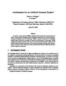
The Human Immune System (HIS) proved to be very successful in protection against different viruses, bacteria and other pathogens that cause damage to the body. It produces immune cells and educates them to detect these damaging entities and to be tolerant to the body’s cells. There are different conceptual and algorithmic models that try to explain how the HIS works [17, 18, 20, 21]. Artificial Immune System (AIS) approaches use these concepts and algorithms for solving analogous problems in artificial systems [26]. We use an AIS approach, as it promises to overcome constraints of traditional misbehavior detection approaches (Section 1.2). We map concepts and algorithms of the HIS to a mobile ad-hoc network and build a distributed AIS system for DSR misbehavior detection. Every node runs the same detection algorithm based on its own observations. The nodes also exchange signals among each other (Figure 1).

Tonsils and adenoids Lymph nodes

AIS

AIS

Lymph nodes

AIS

Thymus

AIS AIS

Spleen Appendix Bone marrow

Peyer’s patches Lymph nodes Lymph vessels

AIS

AIS

AIS - Artificial Immune System

Fig. 1. From the human IS to an AIS: Making DSR immune to node misbehavior.

In order to introduce our specific AIS approach and solutions (Section 1.5), we first explain existing AIS approaches and some problems that are not solved by these approaches (Section 1.4). We define the building blocks of our AIS for routing misbehavior detection and explain how the system works in Section 3. The detailed description of the building blocks and their components is given in Section 4.

4

1.4

S. Sarafijanovi´c and J. Y. Le Boudec

Existing AIS Approaches and Unsolved Problems That We Address Here

Existing AISs [25–28] are mainly based on what is called : self-nonself model of the HIS, negative selection and clonal selection. According to the self-nonself model of the HIS, the HIS cells are produced with aim to not detect molecules and proteins that are predefined (in the thymus) to belong to the body and body’s cells (self), and to detect all the other molecules and proteins (nonself), including those on viruses, bacteria and other pathogens. AIS analogs of the HIS cells are called detectors. A randomly produced detector can recognize one or more elements from an observable universe. For example, a universe is any possible behavior that can be observed for network nodes. A self-nonself-modelbased AIS predefines one part of the observable universe to be self (normal behavior of network nodes, for example). Then it produces the detectors with aim to detect all other elements of the universe, but to not detect those from the self part [3]. The detectors are produced in the process of negative selection: they are generated at random, those that can detect self examples are deleted, and the others are used for the detection. Such detectors are more or less self tolerant, depending on how well self is described by the predefined self examples and whether self is noisy and changing with time. Because of their random nature, the detectors have good coverage of nonself, even if nonself is unknown or changing with time. Negative selection alone is in fact an anomaly detection method. The addition of clonal selection and memory [12–14, 2] provides AISs with ability to adapt to the experienced nonself and to detect it faster and with lower false positives in the future. Clonal selection multiplicates and refines (using random modifications) the detectors that are useful in detections. Detectors that become very specific to the experienced nonself become memory. Memory detectors are long lived and can more easily detect repeated nonself for which they are specific (fast secondary response). Recently, the use of the danger signal model of the HIS has been proposed in the AIS literature [5, 6]. The main idea is to generate a Danger Signal (DS), which correlates the damage experienced by the system to be protected with observed antigens (an antigen is a part of a self or nonself element that can be observed and potentially matched by a detector), and to use this signal as an additional control required by detectors for detection and for clonal selection. This additional control is aimed at decreasing false positive detections. There are still some fundamental problems to be solved in AIS approaches: Eliminating need for preliminary learning in protected environment. Most of the AISs require a set of self examples to be collected in advance in order to start producing detectors. To collect self examples, the system to be protected must be run in a protected environment, in which nonself is not present. In most of the cases in practice, such a protected environment is either inconvenient or impossible to provide. Capability to learn changing self. Even if an initial set of self examples is available, but a dynamic updating of this set is not provided, AISs will not operate correctly if self changes over time. The problem is that detectors produced in the process of negative selection will be self-reactive. False positives caused by these detectors can be decreased by requiring the existence of a correlated danger signal in order to have detection, but this makes AISs more sensitive to the wrong danger signals. Fully reliable

An AIS with Virtual Thymus, Clustering, Danger Signal and Memory Detectors

5

danger signals are often difficult to find in concrete AIS applications, which is probably the reason why the danger signal is only proposed but yet not used in the literature. This would especially be the issue in distributed environments, for example in our misbehavior detection problem. For reliable low false-positives detection, both successful dynamic description of self and danger signal should be used. The problem of dynamic providing of self examples is not solved in the related literature. The only known system that provides dynamic description of self is that of Somayaji and Forrest [4]. Their system achieves tolerance to new normal behavior in an autonomous way, but it works only under the assumption that new misbehavior always shows new patterns that are more grouped in time than new patterns of normal behavior; if the patterns of a new misbehavior are first sparsely introduced in the system, the system will become tolerant to that misbehavior. For their concrete application, as well as for many other AIS applications, such an assumption does not hold. Kim and Bentley [12–14] define and investigate in detail the dynamic clonal selection algorithm. They show that the algorithm enables an AIS to learn changing self if the examples of the current self are provided, but they do not tackle the problem of providing the self examples. We believe that adding a component to an AIS that solves this problem would enable the AIS to autonomously learn about and defend a changing protected system. Mapping from matching to detection. Matching between an antigen and an antibody is not enough to cause detection and reaction in the HIS [18, 19] (antigens are proteins that cover the surface of self and nonself cells; antibodies are proteins produced by the HIS, capable of chemically binding to nonself antigens). The clustering of the matches on the surface of an immune cell and an additional danger signal are required for detection. These additional requirements can be viewed as detection control mechanisms aimed at decreasing false positives. These mechanisms are still not appropriate in existing AISs. The high false-positives detection rate is a common unsolved problem of many AISs, although it seems not to be so with the HIS. 1.5

Our AIS Approach for Protecting Dynamic Self

Our goal is to make an AIS that, analogously to its natural counterpart [16], automatically learns and detects both already encountered and new nonself, but becomes tolerant to any previously unseen self. Our AIS learns the dynamic self, produces the detectors and does the detection using four AIS concepts: “virtual thymus”, “clustering”, “danger signal” and “memory detectors”. Virtual Thymus. “Virtual Thymus” (VT) is a novel concept that we introduce in this paper. It uses observed antigens and generated DSs (the concept of the DS is defined below) and continuously provides self antigen examples that represent the dynamic self of the protected system. It solves the problem of learning a changing self and eliminates the need for a preliminary training in a protected environment. Apart from the negative selection, the way our VT works does not have analog in the existing theories of the HIS. It is important to mention that it is not yet clear to the immunologists how the repertoire of the antigens presented in the thymus during negative selection is formed (see Section 2.1).

6

S. Sarafijanovi´c and J. Y. Le Boudec

Clustering. Clustering is also a novel concept that we introduce in this paper. It maps matches between the detectors and antigens into the detection decisions in a way that constrains false-positive detection probability and minimizes the time until detection under this constraint. The term clustering comes from immunology, where it denotes grouping of matches between antibodies and antigens that is required for recognition of a pathogen. Danger Signal. The Danger Signal (DS) is generated when there is a damage to the protected system. It correlates the damage with the antigens that are in some sense close to the damage, showing that these antigens might be the cause for the damage. We use the DS as a control mechanism for the detection and clonal selection, with the aim to decrease the false positives, which is already proposed but not implemented in the existing AISs. This use of the DS, and the way how it is generated is analogous to the DS and Antigen Presenting Cells (APC) in Matzinger’s model [16] of the HIS. As mentioned above, we also use the DS to implement VT, which is a novel use of the DS. We have to mention that this use of the DS doesn’t have its analog in the existing theories and models of the HIS. Memory Detectors. As already mentioned in Section 1.4, the detectors that prove useful in the detection undergo the clonal selection process and become memory. They provide a fast response to the already experienced nonself. Clonal selection and memory detectors are well investigated in the related literature [12–15].

2 BACKGROUND. 2.1

Background on the Human Immune System

The main function of the HIS is to protect the body against different types of pathogens, such as viruses, bacteria and parasites and to clear it from debris. It consists of a large number of different innate and acquired immune cells, which interact in order to provide detection and elimination of the pathogens [18]. We present a HIS overview based on the self-nonself and the danger models [18, 17]. Functional architecture of the IS. The first line of defense of the body consists of physical barriers: skin and mucous membranes of digestive, respiratory and reproductive tracts. It prevents the body from being entered easily by pathogens. The innate immune system is the second line of defense. It protects the body against common bacteria, worms and some viruses, and clears it from debris. It also interacts with the adaptive immune system, signaling the presence of damage in self cells and activating the adaptive IS. The adaptive immune system educates its cells to be tolerant to the body’s cells, but adapts them to better detect both experienced and previously unseen pathogens. It provides an effective protection against viruses even after they enter the body cells. It memorizes encountered viruses for more efficient and fast detection in the future. The innate immune system consists of macrophages cells, complement proteins and natural killer cells. Macrophages are big cells that are attracted by bacteria to engulf the bacteria in the process called “phagocytosis”. Complement proteins can destroy some

An AIS with Virtual Thymus, Clustering, Danger Signal and Memory Detectors

7

common bacteria. Natural killer cells can kill cells that do not do MHC presentation properly. When there is an attack, the innate cells involved in the response emit signals in order to recruit more immune system cells against the attack. The adaptive immune system consists of two main types of lymphocyte cells. These are B cells and T cells. Both B and T cells are covered with antibodies. Antibodies are proteins capable of chemically binding to nonself antigens (in case of T cells, the antibodies are usually called receptors, and they are never secreted from the cell). Antigens are proteins that cover the surface of self and nonself cells. Whether chemical binding takes place between an antibody and an antigen depends on the complementarity of their three-dimensional chemical structures. If it does, the antigen and the antibody are said to be “cognate”. Because this complementarity does not have to be exact, an antibody may have several different cognate antigens. What happens after binding depends on additional control signals exchanged between different IS cells, as we explain next. B cells repertoire. One B cell is covered by only one type of antibody, but two B cells may have very different antibodies. As there are many B cells (about 1 billion fresh cells are created daily by a healthy human), there is also a large number of different antibodies at the same time. How is this diversity of antibodies created and why do antibodies not match self antigens? The answer is in the process of creating B cells. B cells are created from stem cells in the bone marrow by rearrangement of genes in immature B cells. Stem cells are generic cells from which all immune cells derive. Rearrangement of genes provides diversity of B cells. Before leaving bone marrow, B cells have to survive negative selection in the bone marrow: if the antibodies of a B cell match any self antigen present in the bone marrow during this phase, the cell dies. The cells that survive are likely to be self tolerant. T cells repertoire. B cells are not fully self tolerant, because not all self antigens are presented in bone marrow. Self tolerance is provided by T cells that are created in the same way as B cells, but in the thymus, the organ behind the breastbone. T cells have good self tolerance, because almost all self antigens are presented to these cells during negative selection in the thymus. There are two types of T cells, T helper cells (Th) and T killer cells (CTL). Humoral response. After some antibodies of a B cell match antigens of a pathogen or self cell, that antigens are processed and presented on the surface of the B cell. The presentation is done by Major-Histocompatibility-Complex molecules type II (MHC II). If antibodies of some Th cell bind to these antigens and if the Th cell is activated, it will give costimulation to the B cell and activate it. Some activated B cells start the process of producing many new similar B cells, that will be able to match the pathogen better. This process is called clonal selection. It is explained below. Another activated B cells secret antibodies that opsonize the pathogens, marking them to be engulfed by macrophages and eliminated. The process stops when pathogens are cleared from the body. Some of the B cells produced in the humoral response become memory. They are long lived and ready to react promptly to the same cognate pathogen in the future.

8

S. Sarafijanovi´c and J. Y. Le Boudec

If B cell did not receive the costimulation, it means that the detected antigens are probably self antigens for which the T cells are tolerant. In this last case, the B cell will die together with its self reactive antibodies. The costimulation to the B cells (and their activation) can come from the innate cells as well. B cells can secret antibodies or begin clonal selection without being costimulated, but only in the case when matching between B cell antibodies and antigens is very strong. This occurs with a high probability only for memory B cells. Whereas first time encountered pathogens require a few weeks to be learned and cleared by the IS, the secondary reaction by memory B cells takes usually only a few days. Clonal Selection. In the clonal selection phase, a B cell divides into a number of clones with similar but not strictly identical antibodies. Statistically, some clones will match the pathogen that triggered the clonal selection better than the original B cells and some will match it worse. If the pathogens whose antigens triggered clonal selection are still present, they will continue to trigger cloning new B cells that match the pathogen well. The process continues reproducing B cells more and more specific to present pathogens. B cells that are specific enough become memory B cells and do not need costimulation. This is a process with positive feedback and it produces a large number of B cells specific to the presented pathogen. Cellular Response. This is the response by CTL cells against pathogens that manage to enter body’s cells, i.e. against viruses. MHC type I molecules of a body cell sample and present antigens that are inside the cell. If these antigens are recognized by CTL receptors, and if there is a Th cell that costimulates this antigen recognition, CTL is activated and it governs the infected body cell to die. Activated CTLs proliferate and respond to the viruses. Most of the CTL cells are programmed and die after doing their job, but some of them become memory CTLs. Memory CTLs are long lived, do not require costimulation by Th cells in order to be activated, and produce fast secondary response to the reinfection by the same or similar virus. Clustering. Recognition of a pathogen by a B or CTL cell requires that the antibodies (receptors) of these cells bind not only one but more antigens from the pathogen simultaneously. This is called clustering. It provides some robustness to false antibodyantigen binding. The Danger Signal is a control used for activating Th cells, the cells that control activation of non-memory B and CTL cells. The danger signal (DS) is generated when there is some damage to self cells, which is usually due to pathogens. As an example, the DS is generated when a cell dies before being old; the cell debris are different when a cell dies of old age or when it is killed by a pathogen. DS is transported to Th by antigen presenting cells (APC). An APC transports some information about antigens found around the place of the damage (that potentiality belong to the pathogen). This information instructs Th cells to costimulate those B or CTL cells that has recognized similar antigens.

An AIS with Virtual Thymus, Clustering, Danger Signal and Memory Detectors

9

Self Presented in The Thymus. The way how the self is provided that is presented during negative selection in the thymus is still an open question in biological research ([18], pages 85-87; [19]): (1) both self and non-self antigens are presented in the thymus; the rules about how antigens can enter the thymus from the blood are unclear; (2) the thymic dendritic cells that present antigens survive for only a few days in the thymus, so they present current self antigens; if a non-self antigen is picked up for presentation during an infection, it will be presented only temporarily; once the infection is cleared from the body, freshly made antigens will no longer present the foreign antigen as self. 2.2

Background on DSR

The dynamic source routing protocol (DSR) is one of the candidate standards for routing in mobile ad-hoc networks [23]. A “source route” is a list of nodes that can be used as intermediate relays to reach a destination. It is written in the data packet header at the source; intermediate relays simply look it up to determine the next hop. DSR specifies how sources discover, maintain and use source routes. To discover a source route, a node broadcasts a route request packet. Nodes that receive a route request add their own address in the source route collecting field of the packet, and then broadcast the packet, except in two cases. The first case is if the same route request was already received by a node; then the node discards the packet. Two received route requests are considered to be the same if they belong to the same route discovery, which is identified by the same value of the source, destination and sequence number fields in the request packets. The second case is if the receiving node is the destination of the route discovery, or if it already has a route to the destination in its cache; then the node sends a route reply message that contains a completed source route. If links in the network are bidirectional, the route replies are sent over the reversed collected routes. If links are not bidirectional, the route replies are sent to the initiator of the route discovery as included in a new route request generated by answering nodes. The source of the initial route request is the destination of the new route requests. The node that initiates original route request receives usually more route replies, each containing a different route. The replies that arrive earlier than the others are expected to indicate better routes, because for a node to send a route reply, it is required to wait first for a time proportional to the number of hops in the route it has as answer. If a node hears that some neighbor node answers during this waiting time, it supposes that the route it has is worse than the neighbor’s route, and it does not answer. This avoids route reply storms and unnecessary overhead. After the initiator of route discovery receives the first route reply, it sends data over the obtained route. While packets are sent over the route, the route is maintained, in such a way that every node on the route is responsible for the link over which it sends packets. If some link in the route breaks, the node that detects that it cannot send over that link should send error messages to the source. Additionally it should salvage the packets destined to the broken link, i.e., reroute them over alternate partial routes to the destination. The mechanisms just described are the basic operation of DSR. There are also some additional mechanisms, such as gratuitous route replies, caching routes from forwarded or overheard packets and DSR flow state extension [23].

10

S. Sarafijanovi´c and J. Y. Le Boudec

3 OVERVIEW OF OUR AIS 3.1

AIS Building Blocks

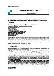
The four main AIS concepts that we use (Virtual Thymus, Clustering, Danger Signal and Memory Detectors) are implemented within the six building blocks (Figure 2), at every network node.

Observed routing protocol events

System To Be Protected (network with routing)

Observed degradation of communication quality (packet loss)

AIS

This Node AIS

Immature detectors

Antigens

Virtual Thymus

Mapping

DS (1)

DS (Danger Signal) Block

Bone Marrow Naive Detectors

DS (3)

Naive Detectors Cloned Detectors

Clonal Selection

Memory Detectors

Other Nodes AIS

Antigens

Danger Signal Exchange Among The Nodes

DS (2)

Clustering

Detection Output

Fig. 2. AIS building blocks in one network node. Note: DS(1), DS(2) and DS(3) are all the same danger signal, indexing only emphasizes three different uses of it.

The Mapping and Danger Signal (DS) blocks are interfaces to the system to be protected and to AISs in other nodes. The mapping block transforms observed routing protocol events into internal AIS representation of the behavior (Antigens). The DS block transforms the experienced degradation of the communication quality of this node into the danger signal, and exchanges the signal with other nodes. The Virtual Thymus (VT) uses danger signal to dynamically select self examples from the collected antigens. It uses the selected self antigens for negative selection of the detectors produced by the Bone Marrow block. The Clonal Selection block multiplies and refines useful detectors, if they get costimulated by the danger signal. The Clustering block defines whether matching between the detectors and the observed antigens results in the detection of the corresponding node or not. The result depends on the numbers of observed and matched antigens for that node, on the types of the detectors that matched (whether they are memory or not), and on the presence of correlated danger signals.

An AIS with Virtual Thymus, Clustering, Danger Signal and Memory Detectors

3.2

11

How The AIS Works.

Here we explain how the AIS works by putting a node equipped with the AIS in the network scenarios typical for invocation of certain blocks or concepts. For the details, please see the pseudo code of the six AIS building blocks (Appendix B) and the values of the used parameters (Table 1 in Section 5). Bootstrap. When a node joins the network for the first time, it does not have any preloaded knowledge or data examples about normal behavior or misbehavior in the network. It starts its AIS in the initial self learning phase. In this phase the node observes antigens and uses the VT to collect self examples. It uses the DS block to provide DSs needed for correct functioning of the VT. In this phase Clonal Selection and Clustering blocks are turned off. This is done in order to avoid initial false positives until the number of the self antigen examples stabilizes. Once the number of self examples reaches a threshold, the node turns on the Clonal Selection and Clustering blocks, i.e., it enters detection phase and stays in this phase all the time. During the detection phase the node continues to observe antigens, produce DSs, and dynamically update self examples. If the node leaves the network and joins it again, it may start with saved self examples and enter detection phase immediately. It is important to notice that there are no assumptions on the behavior of the other nodes during the initial learning phase (some of them may misbehave). Also, the node starts to participate in routing and use the network to communicate already in the initial learning phase. Observing Antigens. The node continuously observes routing protocol events for all its neighbors and temporarily records them within subsequent time intervals of predefined length (a system parameter). Two nodes are neighbors if they are within radio range of each other. Examples of protocol events are route request received, data packet received, data packet forwarded. Protocol events collected for one neighbor within the last time interval are compressed into a compact form, called antigen. The antigen represents the behavior of the observed node in that time interval. The details of mapping from the observed protocol events to the antigens are given in Section 4.1. Generating, Transmitting and Receiving the DS. When a node communicates with another node, it normally receives acknowledgments for its data packets, that are sent by the destination. The danger signal is generated by a node when it experiences a packet loss, i.e., when it does not receive the acknowledgment (packet loss is seen as a damage to the protected system). The DS is then sent over the route on which the packet loss took place, and received by all the nodes that can overhear it. A typical scenario is shown on the Figure 3. The DS contains the information about the (approximate) time of the packet loss, and about the nodes on the route over which the lost packet was sent. So, the receivers of the danger signal are able to correlate it with the collected antigens that are close in time and space (on the same route) to the experienced damage (i.e. to the packet loss). (There is a strong analogy with the HIS, regarding both the way the danger signal is generated and the information it contains; see Section 2.1.)

12

S. Sarafijanovi´c and J. Y. Le Boudec

vF

F

Antigen(B)

F

Packet loss

B

source

S

packet

E

D

DS

DS

A Antigen(S) Antigen(A) + DS

packet

destination

C

Antigen(A) Antigen(B) + DS

B-misbehaving node

Fig. 3. Generating, transmitting and receiving the danger signal (DS): node S is sending data packets to D over an established route; there is a packet dropped by node B; the source S of the packet does not receive the acknowledgment from the destination D; S generates and sends the danger signal over the route on which the loss took place; the nodes that receive the danger signal are A, B, C and E. In this scenario, node F moves away and do not receive the danger signal.

It is possible that the DS is generated even if there is no any misbehavior, because a packet was lost due to a excessive collision of radio signals, or break of the used route due to the mobility, which normally happens in mobile ad hoc networks. Our system is robust to such false DSs, as explained in the next three paragraphs. Use of the DS in The VT: Achieving The Dynamic Self. To define dynamic self in our system, we extend the notion of self from the behavior specified by the routing protocol (DSR, for example) to any interactive node behavior that does not have negative effects on the normal network trafficking, i.e. does not cause packet losses. As a packet loss, we count any case in which the packet does not arrive at the destination, or the acknowledgment from the destination about receiving the packet does not reach the source, or there is a high delay in any of these packets. How the node learns the dynamic self is shown on the Figure 4. Whenever the node observes a new antigen, it sends it towards the thymus with a delay that is large enough to receive all the DSs that could be related to that antigen. If none of potentiality received DSs correlates this antigen to a damage experienced in the network, the antigen is considered as self and passed into the thymus if needed. Once the number of self antigen examples reaches its stable value (it is the end of the initial self learning phase), a new example is added only when an old one leaves the thymus. Producing New Naive Detectors in VT. New naive detectors are produced in the VT all the time in a process of dynamic negative selection. In the initial self learning phase, new random detectors are generated by the Bone Marrow and negatively selected with all collected self antigens. When new self antigen is collected, all existing detectors are negatively selected only with that new self antigen. The detectors are not used for the detection in this initial phase. Note that the method is

An AIS with Virtual Thymus, Clustering, Danger Signal and Memory Detectors

13

Virtual Thymus

Thymus

“Self” Antigens

Delay

Immature detectors

DS

Antigens

DS

Naive Detectors

Fig. 4. Virtual Thymus: Self to be used in the dynamic process of clonal selection is dynamically collected from the observed antigens that are not correlated with any danger signal.

computationally more convenient and not more costly then collecting all self examples and then creating and checking all the detectors. After the initial learning phase, a new self antigen that enters the thymus is used to negatively select only newly created immature detectors, but not those that already passed the negative selection (and became naive). The number of naive detectors stays approximately constant. A naive detector that does not score enough matches to undergo clonal selection dies after a fixed life time (a parameter). In parallel, if the number of naive detectors is smaller then a maximum value (which is a parameter), new naive detectors are generated by the negative selection in the VT. The naive detectors that score many matches and receive costimulations by the DSs for that matches undergo clonal selection and become memory. The detector is first duplicated. One copy becomes a memory detector, while another is hypermutated and becomes new naive detector. Finite-Time Antigen Presentation in The VT and Wrong DSs. A collected self-antigen example is used in the VT for a finite time, then it leaves the VT and is replaced with fresh one. This aging and continuous updating provides the VT with the current version of the “dynamic self”, and makes AIS less sensitive to nonself antigens that are mistakenly selected as self examples (because the DS was mistakenly absent). If a nonself antigen is mistakenly picked up and used to represent self, new naive detectors that match it will not be produced until this antigen leaves the VT. During this time period, the detectors produced before the nonself antigen is picked up are still able to match that and similar antigens. Wrong DSs that are mistakenly or intentionally generated may prevent self antigen to be used as an example. This is not a problem for the VT as there would be other self examples that are collected. It is also possible to counteract misbehaving nodes that try to maliciously generate many fake DSs and prevent other nodes from collecting enough self examples (an attack to the AIS). In our case such a malicious node may be detected because it sends too many DSs, though it should change a path that is not

14

S. Sarafijanovi´c and J. Y. Le Boudec

working for its data packets if it really has a reason to send danger signals (in current AIS simulation this type of misbehavior is not implemented). In general, as this is a known attack specific to VT, a specific predefined detector(s) may be designed for it in a concrete AIS. It is important to note that the joint use of the “dynamic self” and danger signal brings new quality to the robustness of the AIS: false positive matches by detectors are partially compensated by the absence of the danger signal; temporary presence of wrong danger signal does not cause detection if there is no corresponding false positive matching by current detectors whose production was indirectly controlled by danger signals in the past; if the danger signal is currently mistakenly absent to costimulate detection for a nonself antigen, memory detectors for which correct education was assisted by the danger signal in the past can do detection. Matching. Once the detection phase starts, every new observed antigen is checked with the existing detectors for matching. Matches for the antigens observed for one node are temporarily stored and used for clustering and detection (next paragraph). Clustering And Use of The DS for Detection. In order to have detection of a node as misbehaving, our AIS requires more antigens of that node to be matched by the detectors. After every new antigen observed for a node, the matching information is used together with the matching information previously collected for that node within some time window, and a decision is made if there is detection or not (we call this clustering; the term comes from immunology, see Section 2.1). The method is time adaptive. If most of the observed antigens are matched, fewer observations are required for detection. The method may also be tuned to achieve a tradeoff between probability of false-positive detection and the time until detection. The details of the method, including the clustering formula, are given in Section 4.2. In practice, clustering is done for the matches from the finite time window. The size of the window can always be chosen (experimentally) large enough to cover majority of the detection cases. Then, intuitively, the clustering formula approximately holds. The matches by the naive detectors are clustered separately from the matches by the memory detectors. The parameters used for the clustering differ in the two cases as well. As the memory detectors are better educated, they require smaller number of clustered matches for the same false positive probability, and so provide a faster detection. Additional control for decreasing false positives is to require a correlated danger signal for observed antigen, in order to count the matching of that antigen for clustering. Similar methods are used in the HIS, clustering of the matches on the surface of an immune cell and an additional danger signal are required for detection ([18, 19]). Use of The DS for Clonal Selection: Producing Memory Detectors. The detectors that have many matches costimulated by the danger enter the process of clonal selection. They are cloned, i.e. multiplied and randomly modified. The clones that receive costimulation many times (above a threshold) are promoted into memory. Use of Memory Detectors. Analogously to the HIS, our memory detectors do not require the DS to verify their matches to the antigens. Less clustering is also required for

An AIS with Virtual Thymus, Clustering, Danger Signal and Memory Detectors

15

the detection, comparing to the naive detectors and their clones that still did not become memory. Memory detectors are long lived, in order to provide fast response to the experienced misbehavior. As the number of memory detectors is limited, we keep those that are unique. From those that are not unique, we keep last used ones. Concretely, when a new memory detector is created and the number of the existing memory detectors is maximum possible, we choose an old memory detector to delete as follows. We find existing memory detectors that are able to match certain number (that is a parameter) of the latest antigens matched by the new detector before it became memory (these are similar to the new memory detector), and from these we delete the one that is not used for the longest time. If we do not find such similar ones, then we delete the one that is not used for the longest time among all the old detectors. DS is not needed for matches by memory detectors to be counted for the detection. But a systematic absence of DSs for similar antigens matched by a memory detector means that the memory detector is probably reactive to the new self, and it is deleted. For the details of the testing see Appendix B. 3.3

Mapping of HIS Elements to Our AIS

The elements of the natural IS used in our detection system are mapped as follows: – – – –

– – – – – – – – –

Body: the entire mobile ad-hoc network. Self Cells: well-behaving nodes. Non-self Cells: misbehaving nodes. Antigen: (AIS) antigen, which is a sequence of observed DSR protocol events recognized. In the sequence of packet headers and represented by binary strings as explained in Section 3.2 and with the details given in Section 4 (representation is adopted from [14]). Antibody: detector; detectors are binary strings produced in the continuous processes of negative selection and clonal selection; ideally, they “match” non-self antigens (produced by misbehaving nodes) and do not match self antigens. Chemical binding of antibodies to antigens: “matching function” between detectors and antigens, defined in detail in Section 4. Detection: a node detects a neighbor as misbehaving if the node’s detectors match relatively many of the antigens produced by that neighbor (clustering) and if it receives danger signals related to those antigens. Clustering: clustering of matching antibodies on the immune system cell surface is mapped to the clustering of matches between detectors and antigens in time for a given observed node. Aging of the immune cells: finite life time of the detectors Necrosis and apoptosis: packet loss. Danger signal: the danger signal in our framework contains information about the time and nodes correlated with a packet loss. Antigen presenting cell: transmission of the danger signal. Thymus: The virtual thymus is a set of mechanisms that provide (as explained in Section 3.2) the presentation of the current self in the system during the continuous negative selection process.

16

S. Sarafijanovi´c and J. Y. Le Boudec

– Memory cells: memory detectors; detectors become memory if they prove to be useful in detection; they differ from normal detectors by longer lifetime and lower clustering required for detection.

4 Detailed Description of Some Building Blocks 4.1

Mapping behavior to Antigens

The mapping used here was adopted from Kim and Bentley [14]. A node in our system monitors its neighbors and collects one protocol trace per monitored neighbor. A protocol trace consists of a series of data sets, collected on nonoverlapping intervals during the activity time of a monitored neighbor. One data set consists of events recorded during one time interval of duration ∆t (∆t = 10s by default), with an additional constraint to maximum Ns events per a data set (Ns = 40 by default). Data sets are then transformed as follows. First, protocol events are mapped to a finite set of primitives, identified with labels. In the simulation, we use the following list: A= RREQ sent B= RREP sent C= RERR sent D= DATA sent and IP source address is not of monitored node E= RREQ received F= RREP received G= RERR received H= DATA received and IP destination address is not of the monitored node A data set is then represented as a sequence of labels from the alphabet defined above, for example l1 = (EAFBHHEDEBHDHDHHDHD,..) Second, a number of “genes” are defined. A gene is an atomic pattern used for matching. We use the following list: Gene1= Gene2= Gene3= Gene4=

#E in sequence #(E*(A or B)) in sequence #H in sequence #(H*D) in sequence

where #(’sub-pattern’) is the number of the sub-patterns ’sub-pattern’ in a sequence, with * representing one arbitrary label or no label at all. For example, #(E*(A or B)) is the number of sub-patterns that are two or three labels long, and that begin with E and end with A or B. The genes are used to map a sequence such as l1 to an intermediate

An AIS with Virtual Thymus, Clustering, Danger Signal and Memory Detectors

17

representation that gives the values of the different genes in one data set. For example, l1 is mapped to an antigen that consists of the following four genes:
l2 = 3 2 7 6

The genes are so defined that, in the case of normal behavior, the values of different genes are correlated to each other for some pairs of the genes. Some of the pairs lose the correlation if they represent misbehavior. This enables differentiation between normal behavior and misbehavior in the space of all antigens, and enables the detectors that cover misbehavior but not normal behavior to be created. Finally, a gene value is encoded on 10 bits as follows. The range of a gene values that are below some threshold value is uniformly divided on 10 intervals. The position of the interval to which the gene value belongs gives the position of the bit that is set to 1 for the gene in the final representation. The threshold is expected to be reached or exceeded rarely. The values above the threshold are encoded as if they belong to the last interval. Other bits are set to 0. For example, if the threshold value for all the four defined genes is equal to 20, l2 is mapped to the final antigen format: l3 = 0000000010 0000000010 0000001000 0000001000




There is one antigen such as l3 every ∆t seconds, for every monitored node, during the activity time of the monitored node. 4.2

Clustering

Assume we have collected n antigens for the monitored node. Let Mn be the number of antigens (among n) that are matched by detectors. Let θmax be a bound on the probability of false-positive matching (matching a self antigen) that we are willing to accept, i.e. the antigens of well-behaving nodes are matched by detectors with a probability that is less or equal than θmax . We determine a good value by pilot simulation runs (θmax = 0.06). Let α (=0.001 by default) be the false-positive detection that we target. We detect the monitored node (classify it as misbehaving) if r ξ(α) 1 − θmax Mn > θmax (1 + √ ) (1) n θmax n where ξ(α) is the (1−α)-quantile of the normal distribution (for example, ξ(0.0001) = 3.72). As long as Equation (1) is not true, the node is classified as well-behaving. With √ . The derivation of Equadefault parameter values, the condition is Mnn > 0.06 + 0.88 n tion (1) is given in the Appendix A.

5 Performance Analysis 5.1

Analyzed Factors and Experiments

We analyze the effects of turning on/off complete components of the system on its performance metrics defined in the next section. Concretely, we analyze the effects of:

18

S. Sarafijanovi´c and J. Y. Le Boudec

(1) substitution of the preliminary learning phase in a protected environment by the virtual thymus, in case of stationary normal behavior; protected environment means that misbehavior is absent from the network; (2) use of the danger signal for detection control; (3) use of memory detectors; (4) substitution of the preliminary learning phase in the protected environment by the virtual thymus, in the case of normal behavior that changes with time. The changing self is implemented by increasing the amount of the data generated by the nodes at the middle of the simulation (after 30 minutes of simulated time). Clustering is used in all the experiments, as we already have shown its advantage over simple matching in [2]. The values of the system parameters used in the simulation are given in Table 1. The same default values are used in all the experiments. We have found the default values by pilot runs. To learn about the parameters, study the pseudo code of the AIS building blocks (Appendix B) and how the AIS works (Section 3.2). Table 1. AIS Parameters Parameter Default Value AntigenCollectionTime 10 s DelayBufferSizeMax 1200 AntigenTowardsVTMin 70 s StoringTimeDS 11 s AntigPresentTimeVT 250 s MaxNumberOfAntigensVT 1200 MaxNumberNaive 1000 MaxNaiveTime 500 s ThresholdCS 20 ProbaPerBit 0.08 MemoryGroupingParameter 1 MemoryTestTriger 15 NumberOfTestSetsMax 30 MemoryDetTestSize 20 MemoryConfidenceMax 0.5 DetByMemoryTimeWindow 18 s DetByNaiveTimeWindow 40 s ThetaMemory 0.01 AlphaMemory 0.0001 ThetaNaive 0.06 AlphaNaive 0.0001

5.2

Performance Metrics

The metrics we use are: (1) time until detection of a misbehaving node; (2) true-positive detection, in form of the distribution of the number of nodes which detect a misbehaving node; (3) false-positive detection, in form of the distribution of the number of nodes

An AIS with Virtual Thymus, Clustering, Danger Signal and Memory Detectors

19

which detect a well-behaving node. The metrics are chosen from a reputation system perspective; we see the use of a reputation system [9] as a way to add a reactive part to our AIS. 5.3 Simulation: General Settings and Assumptions The simulation is done in Glomosim network simulator [22]. There are 40 nodes in the simulation, of which 5-20 nodes are misbehaving. Mobility is the random way point, speed is 1m/s, without pauses. The simulation area is 800x1000 m, and the radio range is 355 m. A misbehaving node exhibits both types of misbehavior: 1) it does not forward data packets or 2) it does not answer or forward route request messages; when a misbehaving node has a chance to misbehave, it does it with certain probability (0.6 by default), that is also a parameter. Note that the clustering rule given by Equation (1) holds for an infinite time simulation, in which every misbehaving node is eventually detected after a long time (zero false negatives) buy every other node in the network (because of the finite simulation area and RWP mobility). When we stop the simulation, for every encountered and not yet detected misbehaving node we count one false negative. 5.4

Simulation Results

0.6 0.5

200 150 100 50

0.4

0.5 5 misbehaving nodes 10 misbehaving nodes 20 misbehaving nodes

0.3 0.2

0 0

5

10

15

20

0.3 0.2 0.1

0.1

0

0 0 1 2--3 4--7 8--15 16--39 number of nodes which detected a misbehaving node

number of misbehaving nodes

5 misbehaving nodes 10 misbehaving nodes 20 misbehaving nodes

0.4

probability

250

probability

time until detection [s]

All the results are average values of 20 runs, with 90 % confidence intervals for the mean values.

0

1

2--3

4--7

8--15 16--39

number of nodes which detected a well-behaving node

0.5

0.6 0.5

250 200 150 100

0.4 0.3 0.2

50

0.1

0

0

0

5

10

15

number of misbehaving nodes

20

5 misbehaving nodes 10 misbehaving nodes 20 misbehaving nodes

5 misbehaving nodes 10 misbehaving nodes 20 misbehaving nodes

0.4

probability

300 probability

time until detection [s]

(a) (b) (c) Fig. 5. Use of the preliminary learning phase: (a) time until detection, (b) correct detections and (c) misdetections.

0.3 0.2 0.1 0

0

1 2--3 4--7 8--15 16--39 number of nodes which detected a misbehaving node

0

1 2--3 4--7 8--15 16--39 number of nodes which detected a well-behaving node

(a) (b) (c) Fig. 6. Use of the virtual thymus instead of the preliminary learning phase: (a) time until detection, (b) correct detections and (c) misdetections.

S. Sarafijanovi´c and J. Y. Le Boudec 0.6

1 5 misbehaving nodes 10 misbehaving nodes 20 misbehaving nodes

0.5

250 200 150 100

0.4 0.3 0.2

50

0.1

0

0

0

5

10

15

20

probability

300 probability

time until detection [s]

20

5 misbehaving nodes 10 misbehaving nodes 20 misbehaving nodes

0.8 0.6 0.4 0.2 0

0

25

number of misbehaving nodes

0 1 2--3 4--7 8--15 16--39 number of nodes which detected a well-behaving node

1 2--3 4--7 8--15 16--39 number of nodes which detected a misbehaving node

1

0.6 5 misbehaving nodes 10 misbehaving nodes 20 misbehaving nodes

probability

0.5 0.4 0.3 0.2

0.6 0.4 0.2

0.1

0

0

0

5 10 15 20 number of misbehaving nodes

5 misbehaving nodes 10 misbehaving nodes 20 misbehaving nodes

0.8

probability

140 120 100 80 60 40 20 0

0 1 2--3 4--7 8--15 16--39 number of nodes which deteceted a well-behaving node

0 1 2--3 4--7 8--15 16--39 number of nodes which detected a misbehaving node

(a) (b) (c) Fig. 8. Use of memory detectors: (a) time until detection, (b) correct detections and (c) misdetections. 0.6

250

0.5

200 150 100

PLF VT

50 5

10

15

20

number of misbehaving nodes

0.4 0.3 0.2

25

5 misbehaving nodes 10 misbehaving nodes 20 misbehaving nodes

0.5 0.4 0.3 0.2 0.1

0.1

0 0

0.6

5 misbehaving nodes 10 misbehaving nodes 20 misbehaving nodes

probability

300

probability

time until detection [s]

time until detection [s]

(a) (b) (c) Fig. 7. Use of the danger signal for detection decision making: (a) time until detection, (b) correct detections and (c) misdetections.

0

0 0

1

2--3

4--7

8--15 16--39

PLF: number of nodes which detect a well behaving node

0

1

2--3

4--7

8--15

16--39

VT: number of nodes which detect a well behaving node

(a) (b) (c) Fig. 9. Virtual thymus versus preliminary learning phase, the effect of change of normal behavior during the use of the AIS: (a) time until detection, (b) misdetections: preliminary learning phase, (c) misdetections: virtual thymus.

Virtual thymus versus preliminary learning phase in the protected environment: From the Figures 5 and 6 we see that the preliminary learning phase can be substituted by the virtual thymus. Time until detection and the false positives are similar in both cases, while the false negatives are slightly worse in the case with the virtual thymus. This result proves that VT enables the system to learn the protected system self instead of using provided self examples. The danger signal used for detection control has a large impact in decreasing false positives (Figures 7(c) and 8(c)). The use of the memory detectors significantly decreases the time until detection (Figure 8(a)), and also improves true-positive detection (Figures 7(b) and 8(b)). Such impact of the memory is already shown in the related literature [13, 2]. In our case it is the direct consequence of the lower value of the clustering parameter Θmax used for memory detectors (compared to the naive detectors).

An AIS with Virtual Thymus, Clustering, Danger Signal and Memory Detectors

21

Better response to evolving self: From Figure 9 we see that the VT outperforms the solution with the preliminary learning phase in the case of self that has changed during the simulation. For the preliminary learning phase solution, false positive probability increased substantially and become larger then for the VT solution, when the stable normal behavior is substituted by the normal behavior that changes in the middle of the simulation. The reason is that with the preliminary learning phase the initial set of self examples is continued to be used for the negative selection after the self has changed. With VT, examples of new self are learned after the changing point, which directly impacts the false positives.

6 Conclusions From our results we conclude that the examined mechanisms: the virtual thymus, the clustering, the danger signal and the use of memory detectors can be successfully applied to our problem. The use of the “virtual thymus” brings two qualitative advantages compared to the standard AIS: (1) it eliminates the need for the preliminary learning phase in the protected environment, i.e., enables use of the AIS in applications for which a protected environment is not possible; (2) it provides the AIS with the ability to learn self that can change with time; this provides smaller false positives comparing to the case with preliminary training phase, as shown in our experiment (in which self changes in the middle of the simulation). Clustering achieves low false positives by increasing the time until detection, but this price is paid only when a misbehavior is experienced for the first time. The later encounters are solved faster by the memory detectors that require less clustering. We find a simple danger signal in our system, and show how it is useful in controlling detection decisions (decrease of false positives). We also show the use of the DS to implement the VT (the central component of our solution).

7 Discussion and Future Work We expect that the combination of the four concepts bring some additional advantages that have not been analyzed by the simulation. As explained in Section 3.2, in cases of not previously seen self, the self-learning ability of the virtual thymus should improve robustness of the self-tolerance to the wrong danger signals, compared to the thymus with the predefined self examples collected in the preliminary learning phase. This feature is especially important in applications in which a reliable danger signal is difficult to provide (this is the case with our system, see Section 3.2). The effect of wrong danger signals caused by misbehaving nodes and impact of the VT on this effect are not experimentally evaluated here, and it remains as future work. But we should mention that even though wrong DSs (both missing and incorrect) are inherently present (they are not intentionally generated) in our system, the AIS still works well. We have defined the genes manually, in the design phase. It is possible to automate this process by calculating the correlations of automatically generated gene-candidate

22

S. Sarafijanovi´c and J. Y. Le Boudec

pairs on an observed self behavior. Gene candidates can also be formed automatically from the set of observable protocol events. Our solution for collecting self behavior examples in an unprotected environment makes this method more promising. As future work, we also plan to implement the automatic generating of genes, and to better analyze the impact of joint and separate uses of the concepts used in this paper. More detailed experimental analysis is needed to evaluate separately the effects of aging and DS used in the VT on the AIS learning ability and dynamics. We also plan to test the set of algorithms used in our AIS on a standard data set, for example on the data set used in [12–14], and especially evaluate impact of VT and its parameters on the learning ability of the algorithms set.

References 1. J. Y. Le Boudec and S. Sarafijanovic. An Artificial Immune System Approach to Misbehavior Detection in Mobile Ad-Hoc Networks. Proceedings of Bio-ADIT 2004, Lausanne, Switzerland, January 2004, pp. 96-111. 2. S. Sarafijanovic and J. Y. Le Boudec. An Artificial Immune System Approach with Secondary Response for Misbehavior Detection in Mobile Ad-Hoc Networks. TechReport IC/2003/65, EPFL-DI-ICA, Lausanne, Switzerland, November 2003. 3. S. A Hofmeyr and S. Forrest ”Architecture for an Artificial Immune System”. Evolutionary Computation 7(1):45-68. 2000. 4. A. Somayaji and S. Forrest ”Automated Response Using System-Call Delays.” Proceedings of the 9th USENIX Security Symposium, The USENIX Association, Berkeley, CA (2000). 5. U. Aickelin and and S. Cayzer: “The Danger Theory and Its Application to Artificial Immune Systems”, Research Report HPL-2002-244, HP Labs, Bristol, UK, 2002. 6. Aickelin, U., Bentley, P., Cayzer, S., Kim, J. and McLeod, J. (2003) Danger Theory: The Link between AIS and IDS? In Timmis, J., Bentley, P. J. and Hart, E. (Eds) Proc of the Second International Conference on Artificial Immune Systems (ICARIS 2003). Springer LNCS 2787. pp. 147-155. 7. Sergio Marti, T.J. Giuli, Kevin Lai, and Mary Baker. Mitigating routing misbehavior in mobile ad hoc networks. In Proceedings of MOBICOM 2000, pages 255–265, 2000. 8. Yongguang Zhang and Wenke Lee. Intrusion detection in wireless ad-hoc networks. In Mobile Computing and Networking, pages 275283, 2000. 9. S. Buchegger and J.-Y. Le Boudec. A Robust Reputation System for Mobile ad hoc Networks. Technical Report, IC/2003/50, EPFL-DI-ICA, Lausanne, Switzerland, July 2003. 10. S. Buchegger and J.-Y. Le Boudec. Performance Analysis of the CONFIDANT protocol: Cooperation of nodes - Fairness In Distributed Ad-Hoc Networks. In Proceedings of MobiHOC, IEEE/ACM, Lausanne, CH, June 2002. 11. S. Buchegger and J.-Y. Le Boudec. The Effect of Rumor Spreading in Reputation Systems for Mobile Ad-hoc Networks. In Proceedings of WiOpt ‘03: Modeling and Optimization in Mobile, Ad Hoc and Wireless Networks, Sophia-Antipolis, France, March 2003. 12. Kim, J. and Bentley, P. J. (2001), ”Towards an Artificial Immune System for Network Intrusion Detection: An Investigation of Clonal Selection with a Negative Selection Operator” , the Congress on Evolutionary Computation (CEC-2001), Seoul, Korea, pp.1244-1252, May 27-30, 2001. 13. Kim, J. and Bentley, P. J. (2002), ”Immune Memory in the Dynamic Clonal Selection Algorithm.” , Proceedings of the First International Conference on Artificial Immune Systems (ICARIS) Canterbury, pp.57-65, September 9-11, 2002.

An AIS with Virtual Thymus, Clustering, Danger Signal and Memory Detectors

23

14. Kim, J. and Bentley, P. J. (2002), ”A Model of Gene Library Evolution in the Dynamic Clonal Selection Algorithm” Proceedings of the First International Conference on Artificial Immune Systems (ICARIS) Canterbury, pp.175-182, September 9-11, 2002. 15. De Castro, L. N. and Von Zuben, F. J. (2002), ”Learning and Optimization Using the Clonal Selection Principle”, IEEE Transactions on Evolutionary Computation, Special Issue on Artificial Immune Systems, 6(3), pp. 239-251. 16. P. Matzinger. Tolerance, Danger and the Extended Family. Annual Review of Immunology, 12:991-1045, 1994. 17. P. Matzinger. The Danger Model in it’s Historical Contex. Scandinavian Journal of Immunology, 54:4-9, 2001. 18. L.M. Sompayrac. How the Immune System Works, 2nd Edition. Blackwell Publishing, 2003. 19. Richard A. Goldsby, Thomas J. Kindt, Barbara A. Osborne, Janis Kuby: Immunology, 5th edition, W. H. Freeman and Company, 2003. 20. Bretscher P., Cohn M. A theory of self-nonself discrimination. Science 169, 1042-1049, 1970. 21. Burnet F. The Clonal Selection Theory of Acquired Immunity, Vanderbilt University Press, Nashville, TN, 1959. 22. Xiang Zeng, Rajive Bagrodia, and Mario Gerla. Glomosim: A library for parallel simulation of large scale wireless networks. Proceedings of the 12th workshop on Parallel and Distributed Simulations-PDAS’98, May 26-29, in Banff, Alberta, Canada, 1998. 23. D.B. Johnson and D.A. Maltz. The dynamic source routing protocol for mobile ad hoc networks. Internet draft, Mobile Ad Hoc Network (MANET) Working Group, IETF, February 2003. 24. G. Iannaccone C.-N. Chuah, R. Mortier, S. Bhattacharyya, C. Diot. Analysis of Link Failures in an IP Backbone. Proceeding of IMW 2002. ACM Press. Marseille, France. November 2002. 25. Ishida Y. Immunity-Based Systems: A Design Perspective. Springer-Verlag, 2004. 26. Leandro N. de Castro and Jonathan Timmis, Artificial Immune Systems: A New Computational Intelligence Approach, Springer Verlag, Berlin, 2002. 27. Dasgupta D. Artificial Immune Systems and Their Applications. Springer-Verlag, Inc. Berlin, January 1999. 28. De Castro, L. N. and Von Zuben, F. J. (1999), Artificial Immune Systems: Part I Basic Theory and Application, Technical Report RT DCA 01/99.

A Derivation of Equation (1) We model the outcome of the behavior of a node as a random generator, such that with unknown but fixed probability θ a data set is interpreted as suspicious. We assume the outcome of this fictitious generator is iid. We use a classical hypothesis framework. The null hypothesis is θ ≤ θmax , i.e., the node behaves well. The maximum likelihood ratio test has a rejection region of the form {Mn > K(n)} for some function K(n). The function K(n) is found by the type-I error probability condition: P{Mn > K(n)}|θ) ≤ α, for all θ ≤ θmax , thus the best K(n) is obtained by solving the equation P({Mn > K(n)}|θmax ) = α The distribution of Mn is binomial, which is well approximated by a normal distribution with mean µ = nθ and variance nθ(1 − θ). After some algebra this gives K(n) = √ p nξ θmax (1 − θmax ) + nθmax , from which Equation (1) derives immediately.

24

S. Sarafijanovi´c and J. Y. Le Boudec

B Pseudo Code of The Six AIS Building Blocks //All the blocks execute in parallel //In our case, this is implemented using continues-time event based simulation //Every Send() has a corresponding Receive() in another block(s) // Mapping block Initialize the variables; set timerMB=0; While (TRUE){ if (timerMBAntigenTowardsVTMin)replace the oldest one; else drop the antigen; }//end Accept...() Drop antigens from the Buffer if delayed more then AntigPresentTimeVT; Drop antigens from the buffer if correlated with currently stored DSs; if (phaseVT==Stationary){ Delete the antigens from the VT that are presented longer then AntigPresentTimeVT(){ do not delete more then currentNumberOfAntigensInDelayBuffer; delete the oldest ones; }//end Delete...() while (numberOfAntigensInVT