Nonlin. Processes Geophys., 15, 1013–1022, 2008 www.nonlin-processes-geophys.net/15/1013/2008/ © Author(s) 2008. This work is distributed under the Creative Commons Attribution 3.0 License.
Nonlinear Processes in Geophysics
An assessment of Bayesian bias estimator for numerical weather prediction J. Son1 , D. Hou2 , and Z. Toth3 1 Numerical
Prediction Center KMA, Seoul, Korea Modeling Center/NCEP/NWS/NOAA and SAIC, Washington DC, USA 3 Environmental Modeling Center/NCEP/NWS/NOAA, Washington DC, USA 2 Environmental
Received: 24 April 2008 – Revised: 6 November 2008 – Accepted: 6 November 2008 – Published: 16 December 2008
Abstract. Various statistical methods are used to process operational Numerical Weather Prediction (NWP) products with the aim of reducing forecast errors and they often require sufficiently large training data sets. Generating such a hindcast data set for this purpose can be costly and a well designed algorithm should be able to reduce the required size of these data sets. This issue is investigated with the relatively simple case of bias correction, by comparing a Bayesian algorithm of bias estimation with the conventionally used empirical method. As available forecast data sets are not large enough for a comprehensive test, synthetically generated time series representing the analysis (truth) and forecast are used to increase the sample size. Since these synthetic time series retained the statistical characteristics of the observations and operational NWP model output, the results of this study can be extended to real observation and forecasts and this is confirmed by a preliminary test with real data. By using the climatological mean and standard deviation of the meteorological variable in consideration and the statistical relationship between the forecast and the analysis, the Bayesian bias estimator outperforms the empirical approach in terms of the accuracy of the estimated bias, and it can reduce the required size of the training sample by a factor of 3. This advantage of the Bayesian approach is due to the fact that it is less liable to the sampling error in consecutive sampling. These results suggest that a carefully designed statistical procedure may reduce the need for the costly generation of large hindcast datasets.
Correspondence to: J. Son (
[email protected])
1
Introduction
Statistical methods are widely used to process Numerical Weather Prediction (NWP) products with the aim of improving the forecast. The adjustment of dynamically based (NWP) forecasts with statistical models has a long history. Model Output Statistics (MOS) techniques (e.g. Glahn and Lowry, 1972; Woodcock, 1984; Vislocky and Fritsch, 1995) have been widely used since the 1970s. It improves raw numerical forecasts by reducing model bias and filtering out the unpredictable. These statistical algorithms adjust the raw forecast based on a database of retrospective forecasts, preferably from the same model, and the corresponding observations. The size of the sample of forecast-observation pairs is crucial for the application of these algorithms. As the characteristics of the errors in NWP model output depends on the model used in generating the forecast, a large number of retrospective forecasts must be run prior to implementation of a new model or upgrading of an existing model. As NWP models are continuously improved and periodically upgraded, the cost associated with the generation of a large sample of retrospective forecasts may hinder the application of such statistical post processing algorithms. As an example, Hamill et al. (2004) suggest that full benefit of the MOS approach can be achieved with about 20 years of training data. On the other hand, some statistical methods based on Bayes Theorem (Krzysztofowicz, 1983; Berger, 1985; Bernardo and Smith, 1994) have been developed to process NWP model products. They are able to generate probabilistic forecast from a sample of deterministic NWP model output and the corresponding truth. In contrast to the more traditional statistical approach, these Bayesian methods make use of the information from a much larger, existing sample of the truth (observation or analysis), from which the climatology
Published by Copernicus Publications on behalf of the European Geosciences Union and the American Geophysical Union.
1014
J. Son et al.: An assessment of a Bayesian bias estimator with a synthetic
of the meteorological variable in consideration can be derived. Krzysztofowicz (1999) proposed a Bayesian Processor of Forecast (BPF) which quantifies the uncertainty in terms of probability density function of the real value of the forecast variable, given the raw forecast (NWP model output). By using the climatology distribution of the variable and a statistical relationship between the raw forecast and the verification, BPF can estimate this probability distribution function (pdf) from a relatively small sample of the forecast-truth pairs. In addition, the BPF implicitly corrects the bias in the raw forecast. Despite its sound theoretical basis, BPF is not widely used in the statistical processing of NWP products. This paper provides a preliminary test of the simplest Bayesian algorithm, i.e., that used in bias correction. Most Numerical Weather Prediction (NWP) products are subjected not only to random error but also to systematic error (i.e., bias). By definition, bias is the expected difference between nature and a forecast of nature. Bias arises from the limitations of the numerical models used in the integration (Toth and Pena, 2007), and their estimation and correction are of great interest in both research and forecast operations. Particularly, in the case of longer-lead time forecast, bias correction is essential for correcting model drift in the forecast. Interest in bias estimation and correction has been on the rise in recent years with the emergence of ensemble forecast products, especially those from multi-model ensembles, such as the North America Ensemble Forecast System (NAEFS). Because all forecast systems have their own systematic errors (e.g. Hou et al., 2001) and these errors would cause bias in the first and second moments of the ensemble distribution (Cui et al., 2005), they should preferably be removed before single model ensembles are combined to generate a joint, multi-model ensemble. Removing bias also improves highly quadratic scores, such as the root mean square error (RMSE). There are various schemes of bias estimation (e.g. D´equ´e, 2003; Cui et al., 2005). A good bias estimation scheme has two desired characteristics. First, the estimated bias should converge to the true bias with increasing sample size used in the bias estimation (i.e., should yield an unbiased estimate of the model systematic error). Second, the rate at which the estimated bias approaches the real bias should be high. The second requirement is very important for operational applications, where the NWP model is continuously improved and periodically upgraded. Before each implementation, a retrospective data set needs to be generated to facilitate bias estimation and correction. Faster convergence of the estimated bias to its real value implies a higher quality in bias estimation, leading either to an improved forecast (with a specified size of the training sample), or reduced need for computational resources (with specified accuracy). Therefore, the rate of convergence of bias estimation is the most important issue to be analyzed when a bias correction scheme is assessed. Nonlin. Processes Geophys., 15, 1013–1022, 2008
To assess a bias correction scheme, the use of real observation (or analysis) and forecast data sets accumulated for multiple years at operational forecast centers appears to be the most straightforward. However, such analysis/forecast data sets are typically not available. This is because every forecast model evolves as time goes by and the computer resources for regenerating retrospective forecasts are limited. To avoid this limitation, some studies used either an earlier version (cheaper for run) of an operational model (Hamill et al., 2004), or a simpler model (Gneiting et al., 2005) to generate large training data sets. Although the sample size generated in this manner is larger, it is still insufficient for a rigorous study of the basic issue, i.e. the rate of convergence in the bias estimator, which requires a specification of the climatological mean of the forecast. For this reason, a different methodology is followed in this study, by using synthetically generated time series to represent the truth and forecast. In addition to providing arbitrarily long time series to define the climate, this method rules out the regime dependence of bias, and allows a controlled and detailed analysis of the bias estimation and correction methods for better understanding of their performance. The paper is organized as follows: Sect. 2 introduces the bias estimator corresponding to the BPF and compares it with the commonly used method of empirical bias estimation. Section 3 describes how the synthetic analysis and forecast data are generated. Results from experiments and analytical analysis with the synthetic data set are shown in Section 4, and those from a preliminary test with real NWP forecast in Sect. 5. Finally, a summary and a brief discussion of the results are presented in Sect. 6. 2
Empirical and Bayesian bias estimators
The mean systematic error, or bias, of a forecast system, is typically defined as the statistical expectation of the difference between forecast f and the corresponding truth a, i.e. B = E(f − a) = E(f ) − E(a)
(1)
and empirically estimated (e.g. D´equ´e, 2003; Cui et al., 2005) from a sample of size n n 1X (fi − ai ) Bˆ = n i=1
(2)
In fact, if there is no other information available except the sample of the forecast and analysis (a, f ) pairs, this is the only way to estimate the bias. If n is small and the sample is not representative of the population, Bˆ will be significantly different from the real bias B. In other words, to ensure a reasonable estimation of the bias, a sufficiently large sample and/or some special sampling technique is necessary. However, in operational forecasting, the climate probability distribution function (pdf) of a meteorological variable www.nonlin-processes-geophys.net/15/1013/2008/
J. Son et al.: An assessment of a Bayesian bias estimator with a synthetic is often available with many years of observation or analysis. It is also a common practice in both the traditional MOS approach and the Bayesian approach (e.g. Krzysztofowicz, 1999) to assume that the forecast f is the sum of a function of the verification a, denoted by G(a), the constant bias B, and a random error ε independent of the truth a and with zero mean, or mathematically, f = G(a) + B + ε
(3)
An assumption behind Eq. (3) is that the expected value of G(a) is the same as that of the analysis a itself, i.e. E[G(a)] = E(a).
(4)
By considering Eq. (4), the bias B can be expressed as the expected value of the difference between f and G(a), i.e. B = E[f − G(a)]
(5)
And can be estimated from a sample of (f , a) pairs as n 1X Bˆ = [fi − G(ai )] n i=1
(6)
Since E(ε)=0, G(a) is the expected value of (f −B) with given a, i.e. G(a) = E[(f − B)|a]
(7)
and it reflects the statistical relationship between the forecast and the verification. In addition, the first moment of the climate pdf of the analysis, E(a), is used in defining G(a). Therefore, Eq. (6) is the same as the bias estimated by BPF (Krzysztofowicz, 1999) discussed in section 1. As the Bayes Theorem is applied implicitly by using E(a), Eq. (6) is referred as a Bayesian estimator of bias B, in contrast to the empirical bias estimator Eq. (2). An advantage of the Bayesian Bias Estimator (BBE) over the Empirical Bias Estimator (EBE) is that its accurate form Eq. (5) holds not only for the expected value, but also for the conditional expected value, given analysis a, i.e., B = E[{f − G(a)}|a]
(8)
Equation (8) can be easily proved by noting that f −G(a)=B+ε and ε is a random number with 0 mean and independent of the truth a. This property of BBE indicates that the bias B can be accurately estimated by using only a subsample of (a, f ) pairs with a specific value or a small range of values of analysis a, instead of a large sample spanning all of the possible values of a. Consequently, it can be used to increase the rate of convergence in bias estimation and hence reduce the required sample size if a specific accuracy is required. The application of BBE in Eq. (6) requires specifying function G(a). With both the traditional MOS approach and the Bayesian Forecast Processor (Krzysztofowicz, 1999), a linear relation is commonly assumed. As this assumption is www.nonlin-processes-geophys.net/15/1013/2008/
1015
valid in most cases, it is also accepted in this study, although other functions, such as logistic function, can be used. To satisfy Eq. (4), the following linear function is the most natural choice: G(a) = α[a − E(a)] + E(a)
(9)
Note that this is different from the linear assumption in traditional MOS techniques in that the climatological information of the truth, E(a), is employed. It will be noted later that this distinction is very important. With this linear function, Eq. (3) takes the form of f = α[a − E(a)] + B + E(a) + ε
(10)
and, with an estimation of the slope α the BBE in Eq. (6) becomes n 1X Bˆ = [fi − α(a ˆ i − E(a))] − E(a) n i=1
(11)
With the traditional MOS approach, E(a) is unknown or not used. When the mean values of f and a are required (as in bias correction) they are often substituted with an estimation from the sample mean. It can be shown that, with this type of substitution, the BBE in Eq. (11) decays to EBE in Eq. (2). Therefore, the difference between BBE and EBE is not only in the forms of formulation, but also in the nature of the methodology. While the traditional MOS approach, including EBE, adjusts the forecast f based only on the available sample of (a, f ) pairs, BBE uses some information of the truth from the whole population. When there is only a partial sample, the difference is significant. For example, when the forecast skill is very low (α=0), EBE in Eq. (2) adjusts the forecasts to the sample mean while BBE in Eq. (11) adjust them towards to the climatological mean. For convenience in calculation and discussion, the model can be further simplified by denoting b=B+(1−α)E(a) and rewriting Eqs. (10) and (11) as f = αa + b + ε
(12)
and n 1X bˆ = (fi − αa ˆ i) n i=1
(13)
As in the traditional MOS approach, the intercept b of the linear function in Eq. (12) is not the bias defined in Eq. (1) and a bias estimation has to be obtained by adding (α−1)E(a) to the result of Eq. (13). The real simplification is by assuming E(a)=0, or working in normal space. For this special case, b is the bias defined in Eqs. (1) and (13) is the Bayesian Bias Estimator, while the Empirical Bias Estimator in Eq. (2) becomes n 1X (fi − ai ) bˆ = n i=1
(14)
Nonlin. Processes Geophys., 15, 1013–1022, 2008
1016
J. Son et al.: An assessment of a Bayesian bias estimator with a synthetic 3.2
Fig. 1. Autocorrelation coefficient (line) and Partial autocorrelation coefficient (histogram) as a function of time lag (days), calculated from the time series of 40 years of daily reanalysis of 2 m temperature at 37.5 N, 117.5 W.
In this article, calculation and discussion are performed in normal space with Eq. (12) as the linear model, and Eqs. (14) and (13) used as EBE and BBE, respectively. The results can be easily extended to the original space. However, when comparing the two estimators, one should keep in mind that BBE has a general form of Eq. (11) and its usage requires the information of the climatological mean of the truth. 3 3.1
Generation of the synthetic data set General considerations
The synthetic data set used in this study seeks to represent the truth with an arbitrarily long time series resembling the major characteristics of the observation, and express its relationship to the forecast with an analytical formula. Linear models are commonly used in the traditional MOS approach and the Bayesian processor (Krzysztofowicz, 1999), and this practice is followed in this study. As can be seen later, further simplification is made by working in a standard space and unit variance will be specified for both the truth and the forecast. While observation is widely used to represent the truth, objective analysis (which, in addition to the observation, uses the same NWP model as used to generate the forecast) is more commonly used in the major operational centers for model verification and calibration. With this in mind, the truth used in this study is based on real analysis and referred as synthetic analysis, or simply analysis. As this study is focused on the problem of bias correction, or the adjustment of the first moment, the adjustment of the second and higher moments of the probabilistic distribution is ignored. Therefore, the corrected forecast will have the same variance as the truth.
Nonlin. Processes Geophys., 15, 1013–1022, 2008
Synthetic analysis
To represent the truth, a synthetic analysis data set was generated based on the statistics from the National Centers for Environmental Prediction (NCEP) – National Center for Atmospheric Research (NCAR) reanalysis (Kalnay et al., 1996). The reanalysis data set consists of daily analyses, from January 1959 December 1999, for a number of near-surface and upper air variables on a 2.5×2.5 latitude/longitude global grid. Temperature at 2 m height at the grid point 37.5 N, 117.5 W (near Fresno, California) is used for this study. The selection of this point is arbitrary but comparisons with other grid points suggest that the generated time series is representative of mid-latitude regions of North America. To focus on the basic characteristics of bias estimation methods, it is useful to disregard the fluctuations related to the annual cycle. Therefore, the reanalysis time series is standardized by subtracting climate mean from each temperature value and then divided by the standard deviation. Both the climate mean and the standard deviation are calculated from the 40-year (1959–1998) climate data for the Julian day of the year corresponding to the date under consideration. After removing the annual cycle by standardization, the reanalysis time series is used to determine the parameters of an ARMA model, which is then applied to generate the synthetic analysis. An ARMA model (Box and Jenkins, 1976; Gershenfeld and Weigend, 1994) consists of two parts, an autoregressive (AR) part and a moving average (MA) part, and is usually referred to as an ARMA(p,q) model, where p is the order of the autoregressive part and q is the order of the moving average part. It can be written as xt =
p X i=1
φi xt−i +
q X
θj εt−j + εt
(15)
j =1
where φi and θi are the autocorrelation parameters and the moving average parameters of the model, respectively. The error terms εt are generally assumed to be independent and identically-distributed random variables, sampled from a normal distribution with zero mean and unit variance: εt ∼N (0, 1). To select the proper order p for the autoregression, the Autocorrelation Function (ACF) and the Partial Autocorrelation Function (PACF) (Pourahmadi, 2001) of the normalized reanalysis time series were computed and shown in Fig. 1. It can be seen that the ACF decreases most rapidly between lags of 0 to 10 and the time series has an autocorrelation noticeably different from zero only for lags less than 20. PACF at lag k is defined as the correlation coefficient between Xt and Xt+k that is not accounted for by lags 1 through k−1. For an AR(p) model it drops off to zero after lag p. Therefore, it is more convenient to use PACF in identifying the order p (Quenouille, 1949). The fact that PACF vanishes after lag 3 suggests p=3 is an acceptable choice. However, in order to retain as much information as possible from the www.nonlin-processes-geophys.net/15/1013/2008/
J. Son et al.: An assessment of a Bayesian bias estimator with a synthetic real analysis time series, a conservative selection of p=20 is used. In fact, the resulted time series with p=3 and p=20 are very similar. The order of moving average was selected as q =1, after several tests with higher q showed no significant improvement. The coefficients of the ARMA model in Eq. (15) (with p=20 and q=1) are estimated from the normalized reanalysis time series with a size of 14610, using subroutines in the commercial IMSL Stat/Library from Visual Numerics, Inc. The algorithm is similar to that of Box and Jenkins (1976, pages 498–500). The ARMA(20.1) model is then used to generate an arbitrarily long time series, which is used as the synthetic analysis data set. Figure 2 shows a section of the standardized reanalysis time series (t=1 to 365) and a section of the synthetic analysis time series (t=366 to 730), which is generated by the ARMA(20.1) model fitted to the reanalysis. The two sections are hardly distinguishable from each other. Therefore, we conclude that the synthetic analysis is a good approximation of the standardized reanalysis or observational time series. For convenience of calculation and comparison, the synthetic analysis is slightly adjusted so that its mean over a period of 100 000 days (about 270 years) is exactly 0. Both the standardized reanalysis and the synthetic analysis exhibit variability at various frequencies. Although the annual cycle has been removed, some fluctuations with their frequency lower than the random noise still exist in the synthetic analysis time series. Consequently, the average of the time series over a period of about 100 days or shorter is significantly different from its climate mean (0). For example the periods from t=365 to 465 and t=630 to 730 in Fig. 2 are dominated by positive values. These lower frequency fluctuations in the synthetic analysis time series can be interpreted as quasi-seasonal variations associated with the changes in dominant circulation patterns over seasonal or longer time scales and will be further discussed in Sects. 5 and 6. Finally, by specifying different seed value for the random number generator in running the ARMA model, a number of time series of synthetic analysis a can be generated. They are different from each other but have the same statistics and each of them is called a random case of the synthetic analysis in this study. 3.3
Synthetic forecasts
Consistent with Eq. (12), a synthetic forecast time series f is generated using the following normal-linear model: fi = αai + βei + b
(16)
where 0 < α < 1, β =
p 1 − α2
(17)
1017
Fig. 2. The time series constructed from both the real and synthetic analyses. The section t=1 to 365 is from the standardized reanalysis data, and t=366 to 730 from the synthetic analysis generated with ARMA(20.1).
β in Eq. (17) is necessary for the variance of the synthetic forecast f to match that of the synthetic analysis a. α can be easily shown to be the temporal correlation coefficient between the forecast f and the analysis a in standard space, or the anomaly correlation in the original space. In Krzysztofowitcz (1992) this parameter is referred as Bayesian Correlation Score and shown to be meaningful for comparing alternative forecasts. Murphy and Epstein (1989) also relate it to skill scores. In this study, α is varied between 1 and 0 to roughly represent NWP forecasts with lead times varying between 0 (perfect correlation, and no random error) and 15 days (no correlation and the forecast is dominated by random errors). Before proceeding to testing different bias estimation methods, we assess whether f as defined in Eq. (16) is consistent with the statistics of real NWP forecasts. In particular, we are interested to see whether the operational forecasts are approximately normally distributed with an expected value α α¯ (the sample average of the corresponding analysis multiplied by the correlation between forecast and analysis), given analysis a. This assumption should hold for a larger sample ranging over all possible values of the analysis, and for sub samples of analysis values over a particular range. Operational Global Forecast System (GFS) forecasts of NCEP and the corresponding analysis for the period from April 2004 to August 2005 were used in the latter, more stringent test. Figure 3 shows the histograms of the sub sample of forecasts with corresponding analyses between 3.0 and 4.0 degrees, and the hypothetical normal distribution, for the 3-day and 10-day forecast. It can be seen that the normal distribution roughly fits the histogram for both cases. Chi-square (Conover, 1980; Wilks, 2006) and KolmogorovSmirnov (Conover, 1980) tests were performed to quantify the goodness of fit and the result of Kolmogorov-Smirnov is shown in Table 1. For 13 out of the 16 lead times, the empirical and the theoretical distribution are close to each other, justifying the use of Eq. (16).
e is a random number from a normal distribution with zero mean and unit variance, and the subscript i is the index of the time series. The choice of the relationship between α and www.nonlin-processes-geophys.net/15/1013/2008/
Nonlin. Processes Geophys., 15, 1013–1022, 2008
1018
J. Son et al.: An assessment of a Bayesian bias estimator with a synthetic
ˆ Fig. 4. Bias error, b−b, as a function of sample size n, for a randomly selected case using the EBE (grey) and BBE (black). α=0.3. n 1X bˆ = (fi − αai ) n i=1
Fig. 3. Histogram of the real operational forecast distribution and the hypothetical pdf of the normal distribution N (α a, ¯ σ 2 ) where a¯ is the sample mean of the corresponding analysis, α the forecastanalysis coefficient and σ 2 the sample variance (see the text for details). Table 1. The Kolmogorov-Smirnov test of the goodness of fit for various forecast lead times. D denotes maximum difference between the theoretical and the empirical cumulative distribution functions, and Prob the probability of the statistic exceeding D under the null hypothesis of equality and against the one-sided alternative. The approximation is very close for Prob less than 0.10.
4
Lead time
D
Prob
Lead time
D
Prob
day 1 day 2 day 3 day 4 day 5 day 6 day 7 day 8
0.2786 0.1656 0.1867 0.4537 0.3709 0.4311 0.3959 0.2668
0.0103 0.1934 0.1253 0.0000 0.0003 0.0000 0.0001 0.0150
day 9 day 10 day 11 day 12 day 13 day 14 day 15 day 16
0.2982 0.2944 0.3613 0.2766 0.3145 0.2860 0.2557 0.1246
0.0053 0.0060 0.0004 0.0110 0.0029 0.0080 0.0211 0.3871
Results with the synthetic data set
With the synthetic data set described in Sect. 3, the Bayesian Bias Estimator is Eq. (13) and, if using the specified value of the correlation coefficient, it takes the form of
Nonlin. Processes Geophys., 15, 1013–1022, 2008
(18)
In this section, BBE is compared with EBE defined in Eq. (14), in terms of accuracy of the bias estimate and requirement of sample size for a specified accuracy. For each case of the analysis times series, a forecast time series is generated with a specified α using Eq. (16) and the bias estimation bˆ is calculated from the first n (a, f ) pairs for n=1, 2, 3. . . and so on. This sequential sampling, without skipping, is commonly used in both research and operations of NWP output processing (e.g. Hamill et al., 2004; Cui et al., 2005). b=1 is assumed in the calculations but the results can apply to any value of b because the bias error is independent of the bias level. This can be shown mathematically. For the synthetic forecast used in this study (Eq. 16), the two bias estimators can be generalized by n 1X bˆn = [(α − γ )ai + βei + b] n i=1
(19)
where γ =1 for EBE and γ =α for BBE. From Eq. (19) one can see that n P bˆ − b = n1 [(α − γ )ai + βei + b] − b = =
1 n 1 n
n P i=1 n P
i=1
[(α − γ )ai + βei ] +
1 n
n P
b−b
(20)
i=1
[(α − γ )ai + βei ]
i=1
is independent of b. Figure 4 depicts the error in the estimated bias, b−bˆ as a function of the sample size n in a randomly selected case with α=0.3 (corresponding to lead time of 12 days). The error is characterized by large values and rapid variations with n