determination based on the Stokes-Helmert approach. (Ellmann ... Gravimetric geoid computation by the Stokes integral ... Laboratory, University of Montfort, UK.
An Attempt for an Amazon Geoid Model Using Helmert Gravity Anomaly D. Blitzkow, A.C.O.C. de Matos, I.O. Campos, A. Ellmann, P. Van´ıcˇ ek and M.C. Santos
Abstract This paper describes the computation of a geoid model for the Amazon Basin (GEOAMA) limited by 5◦ N and 10◦ S in latitude and 70◦ W and 50◦ W in longitude. The software package SHGEO developed by the University of New Brunswick, Canada, was used for the calculation. The geoid model was derived by using the following data: digital terrain model SRTM3 (Shuttle Recovery Topography Mission) version 2.0 with 3” grid, the geopotential model EIGEN-GL04S1, degree and order 150, derived from GRACE satellite, and terrestrial gravity data basically observed along the rivers. For GEOAMA validation the longitudinal profiles of some rivers over the basin derived from three geoid models (EGM96, D. Blitzkow Laboratory of Topography and Geodesy, Department of Transportation, University of S˜ao Paulo, EPUSP-PTR, Postal Code 61548, CEP:05424-970, S˜ao Paulo, S˜ao Paulo, Brazil A.C.O.C. de Matos Laboratory of Topography and Geodesy, Department of Transportation, University of S˜ao Paulo, EPUSP-PTR, Postal Code 61548, CEP:05424-970, S˜ao Paulo, S˜ao Paulo, Brazil I.O. Campos Laboratory of Topography and Geodesy, Department of Transportation, University of S˜ao Paulo, EPUSP-PTR, Postal Code 61548, CEP:05424-970, S˜ao Paulo, S˜ao Paulo, Brazil A. Ellmann Department of Transportation, Faculty of Civil Engineering, Tallinn University of Technology, Ehitajate tee 5, 19086 Tallinn, Estonia P. Van´ıcˇ ek Department of Transportation, Faculty of Civil Engineering, Tallinn University of Technology, Ehitajate tee 5, 19086 Tallinn, Estonia M.C. Santos Department of Geodesy and Geomatics Engineering, University of New Brunswick, P.O. Box 4400, Fredericton, NB, Canada E3B 5A3
MAPGEO2004 and EIGEN-GL04C) combined with geodetic heights from 28 GPS stations close to the tide gage stations were used. The results show that GEOAMA is in good agreement with the EGM96, MAPGEO2004 and EIGEN-GL04C profiles and with the average of the main rivers (Solim˜oes and Amazonas) gradient (20 mm/km). MAPGEO2004 has been the official geoid model in Brazil since 2004. It was developed by Brazilian Institute of Geography and Statistics (IBGE) and Surveying and Geodesy Laboratory of the University of S˜ao Paulo (LTG/USP).
Keywords Geoid modeling· GPS· Height· DTM
1 Introduction The Amazon rainforest has been a challenge for scientists that study the dynamics of changes in this area. It is considered the largest hydrographic basin in the world with 6, 110, 000 km2 , extending from the Andes to the Atlantic Ocean, with 6 countries involved and ∼4.7 million km2 (68%) in Brazil (Campos, 2004). The main river has two denominations: from the border of Peru to Manaus, it is called Solim˜oes, and from Manaus to the Atlantic Ocean, it is called Amazonas. In general, the Amazon region is very flat and for this reason the river gradient is very small. In Manaus, for example, the height of the water level during the dry season is only about 12 m above the mean sea level. The vertical reference network in Amazon region is essential for hydrological and hydrodynamical studies, to compile a regional Digital Terrain Model (DTM) and to construct topographic maps.
M.G. Sideris (ed.), Observing our Changing Earth, International Association of Geodesy Symposia 133, c Springer-Verlag Berlin Heidelberg 2009 �
187
188
Nevertheless, due to the lack of roads and the forest density, it is impossible to carry out spirit levelling for establishing a vertical network in the region. An alternative is to use satellite geodesy associated with a geoid model. This paper presents a particular effort to establish the geoid model GEOAMA for the Amazon Basin, limited by 5◦ N and 10◦ S in latitude and 70◦ W and 50◦ W in longitude. GEOAMA was computed using EIGEN-GL04S1 up to degree and order 60 as the reference field. The reduced Helmert mean gravity anomalies in blocks of 5� were estimated in continental areas. For the ocean KMS-2002 satellite altimetry model was used (Andersen and Knudsen, 1998). The digital terrain model SRTM3, version 2, was chosen for computing the new geoid. The processing of the modified Stokes integral was carried out using the Stokes-Helmert’s geoid software (SHGEO), which is a precise scientific package for gravimetric geoid determination based on the Stokes-Helmert approach (Ellmann and Van´ıcˇ ek, 2007). The present effort is involved in the context, of a major project of LTG/USP with GeoForschungsZentrun (GFZ), Germany, and Institut de R´echerche pour le D´ev´eloppement (IRD), France, for hydrological and gravity variations studies in Amazon. The GEOAMA is an advanced version with respect to MAPGEO2004 (IBGE,2004; Lobianco et al., 2005). In fact, MAPGEO2004 was computed using EGM96 up to degree and order 180 as the reference field. The reduced Helmert mean gravity anomalies were estimated in blocks of 10’. For the ocean KMS99 satellite altimetry model was used (Andersen and Knudsen, 1998). The DTM used obtained from the digitalization of topographic maps, combined with GLOBE model (Hasting and Dunbar, 1999), where topographic maps were unavailable had a resolution of 1� × 1� . The processing of the modified Stokes integral was carried out using FFT technique.
D. Blitzkow et al.
and (4) a set of GPS geodetic heights on the levelling network as control points. This data set is reviewed in the sequel.
2.1 Terrestrial Gravity Data The terrestrial gravity data used in this study has been provided by Petrobras (Brazilian oil company). The observations, a total of 98,176 points, were taken basically along-side the Amazon, Solim˜oes and Madeira rivers in the 1960’s. The majority of the data was measured by LaCoste&Romberg gravitymeter with 0.1 mGal accuracy (Lobianco, 2005). Figure 1 shows the spatial distribution of the points within our target area. Note that due to the rainforest there are vast gravity data gaps.
Fig. 1 Gravity data for the Amazon region
2.2 Geopotential Model
The “satellite-only” model EIGEN-GL04S1, developed up to degree 150, was used to generate the long wavelength contribution of the geoid. On the other The following data set was used for the gravimetric hand, EIGEN-GL04C was used to compute the gravity geoid computation and its validation over the Amazon anomaly in the gaps. The latter is a combination of area: (1) free-air gravity anomalies; (2) geopotential GRACE (Gravity Recovery and Climate Experiment) model for computing the long wavelength component and LAGEOS satellite missions plus 0.5◦ × 0.5◦ grid of the geoid and of the gravity anomaly; (3) a high- of gravimetry and altimetry surface data and it is precision DTM for the computation of terrain correc- complete to degree and order 360 in terms of spherical tion and other topographic effects on geoid modeling; harmonic coefficients (F¨orste et al., 2006).
2 Data Set
An Attempt for an Amazon Geoid Model
189
2.3 Digital Terrain Model
3 Geoid Computations
Gravimetric geoid computation by the Stokes integral requires gravity data referred to the sea level. To ensure the harmonicity of the quantities to be downward continued from the topographic surface to the geoid level Helmert’s second condensation method is often applied. A DTM is used to compute the terrain correction and the indirect effect on the geoid. The data gridding is also an important issue. The mean free-air gravity anomalies used in this study were obtained via mean complete Bouguer anomalies by an approach discussed in Jan´ak and Van´ıcˇ ek (2005). For the present study, we have a suitable gridded topography with a grid size of 3�� × 3�� (approximately 90 × 90 m) from SRTM3 version 2. The SRTM heights are referred to the EGM96-derived geoid and the coordinates in the WGS84 reference ellipsoid (Lemoine et al., 1998a; Lemoine et al., 1998b; Hensley et al., 2001; JPL, 2004; Farr et al., 2007). Over the areas with no SRTM3 information available the 30�� × 30�� . DTM2002 topographic model (Saleh and Pavlis, 2002) was used instead. The DTM2002 combines data from GLOBE (Global Land One-kilometer Base Elevation), version 1.0, constructed by NOAA/NGDC (Hasting and Dunbar, 1999), and ACE (Altimeter Corrected Elevation), from Earth and Planetary Remote Sensing Laboratory, University of Montfort, UK. The global ACE model is derived from altimetry data (Johnson et al., 2001). The heights are referred to the Mean Sea Level. The DTM2002 data was thinned down to 90 × 90 m, i.e. the same spatial resolution as adopted by the SRTM3 model.
The SHGEO precise geoid determination software was employed to compute the GEOAMA geoid model. This package has been developed under the leadership of Professor Petr Van´ıcˇ ek at the Department of Geodesy and Geomatics Engineering, University of New Brunswick (UNB), Canada. This software (Ellmann, 2005a,b) uses StokesHelmert method. The gravity anomalies over the entire Earth are required for the geoid determination by the original Stokes formula. In practice, the area of integration is limited to some domain around the computation point, usually circular. The Stokes equation used to compute the geoidal heights (Ellmann and Van´ıcˇ ek, 2007) is N (Ω) = �� R S M (ψ0 , ψ(Ω, Ω � ))Δg(r g , Ω)dΩ � 4π γ0 (φ) Ωψ0 R � 2 Δg h (r g , Ω) 2γ0 (φ) n−1 n M
+
n=2
δV t (r g , Ω) δV a (r g , Ω) + + γ 0(φ) γ 0(φ)
(1)
where � Δg(r g , Ω) = Δg (r g , Ω) − h
M �
� Δgnh (r g , Ω)
(2)
n=2
The geocentric position (r, Ω) of any point can be represented by the geocentric radius r and a pair of geocentric coordinates Ω = (φ, λ), where φ and 2.4 Control Points λ are the geocentric spherical coordinates; R is the mean radius of the Earth. The modified Stokes kernel In the framework of the Hydrology and Geochemistry S M (ψ0 , ψ(Ω, Ω � )) can be computed according to of the Amazon Basin (HiBAm) international research Van´ıcˇ ek and Kleusberg (1987), where ψ(Ω, Ω � ) is the program, there was an attempt to determine the heights spatial geocentric angle between the computation and at various control points (zero of limnimeters scale) integration points; dΩ � is the area of the integration along the Amazon region rivers, with reference to a element. The UNB approach works to minimize the consistent origin (geoid) (Kosuth and Cazenave, 2002; truncation bias, i.e., uses the low-frequency part of Campos, 2004). A total of 28 stations were selected to the geoid described by a global geopotential model carry out GPS observations on Bench Marks (BM) es- and a spheroid of degree M as a new reference tablished for this purpose as close as possible to the surface (Van´ıcˇ ek and Sj¨oberg, 1991) instead of the limnimeters. The GPS/levelling data have been con- Somigliana-Pizzeti reference ellipsoid. The upper limit (M) for the modified Stokes kernel (geopotential nected to the control points by spirit levelling.
190
D. Blitzkow et al.
model) used in this case was set to 60. This option showed good agreement with GPS/levelling data. In the right-hand side of Eq. (1) the first term is the Helmert residual co-geoid. Since the low-degree reference gravity field is removed from the anomalies before the Stokes integration (Eq. (2)), the longwavelength contribution to the geoidal height (Heiskanen and Moritz, 1967), i.e., the reference spheroid must be added to the residual geoid (the second term on the right-hand side of Eq. (1)). The sum of the first and second terms results with Helmert co-geoid. The third term on the right-hand side of Eq. (1) is the primary indirect topographical effect (Martinec, 1993) and the last term is the primary indirect atmospheric effect on the geoidal heights (Nov´ak, 2000). Accounting for the indirect effects is needed to transform the Helmert geoidal heights back into the real space. The gravity anomaly referred to the geoid surface of Eq. (2) (Δg h (r g, Ω)) is obtained by downward continuation. It is solved using the Poisson integral equation (Heiskanen and Moritz, 1967). This equation had originally been designed as a formula for the upward continuation of harmonic quantities. It can be written as (Kellogg, 1929) Δg h (rt , Ω) �� R = K � Δg h (r g , Ω � )dΩ � 4πrt (Ω) Ω � ∈Ω0
corrections to the Helmert gravity anomaly, such as the direct atmospheric effect, the secondary indirect atmospheric effect, ellipsoidal correction for the gravity disturbance and ellipsoidal correction for the spherical approximation. The 5� × 5� grid of the mean free-air gravity anomalies (Fig. 2) was computed from point gravity data. The EIGEN-GL04C derived anomalies were used to fill gaps with no terrestrial gravity data. Over the ocean, the satellite altimetry-derived gravity anomalies (Global Marine Gravity, 2 arcminute) were used. This model was produced by the Geodetic Division of Kort og Matrikelstyrelsen (KMS2002), the National Survey and Cadastre of Denmark, processing Geosat and ERS-1 satellite altimetry data (Andersen and Knudsen, 1998). The computed Amazon geoid model is shown in Fig. 3.
(3)
where K � = K [rt (Ω), ψ(Ω, Ω � ), R] is the spherical Poisson integral kernel (Sun and Van´ıcˇ ek, 1998). Downward continuation is an inverse problem to the Fig. 2 Mean free-air gravity anomalies original Poisson integral. h The term Δg (rt , Ω), on the left-hand side of Eq. (3), is the Helmert gravity anomaly referred to the Earth’s surface; it can be obtained by (Van´ıcˇ ek et al., 1999) Δg h (rt , Ω) = Δg(rt , Ω) + δ At (rt , Ω) 2 δV t (rt , Ω) + δ Aa (rt , Ω) + rt (Ω) 2 δV a (rt , Ω) + εδg (rt , Ω) − εn (rt , Ω) (4) + rt (Ω) The first term on the right-hand of the Eq. (4) is freeair anomaly; the second and third terms are the direct and secondary indirect topographic effects on the gravitational attraction. Other terms are non-topographical Fig. 3 Geoid heights in the Amazon region
An Attempt for an Amazon Geoid Model
191
4 Geoid Validation
Table 2 Statistics among GEOAMA (D) and EGM96 (A), MAPGEO2004 (B) and EIGEN-GL04C (C)
It has been used the 28 control points (limnimeters) available in Amazon (§2.4) with geodetic coordinates (φ, λ, h) referred to the zero of the limnimeter scale. In a first step of the validation, the geoidal height (height anomaly) has been estimated in these points using EGM96 (A) (Lemoine et al., 1998a,b), MAPGEO2004 (B) (Lobianco et al., 2005) and EIGENGL04C (C) (F¨orste et al., 2006) for comparison with GEOAMA (D). Table 1 shows the 28 control points and their respective geoidal height differences among GEOAMA and the three referred models (D-A, D-B and D-C). The statistics are presented in the Table 2. The biggest differences between GEOAMA and EGM96 are close to the Amazonas estuary; Tabatinga and Santo Antonio do Ic¸a in Solim˜oes River (Fig. 4); and Vista Alegre, Novo Aripuan˜a and Humaita in Madeira River (Fig. 5). Looking to the RMS (Root Mean Square) difference, the column D-C shows a smaller value. It means that EIGEN-GL04C fits much
Mean RMS Maximum Minimum
D-A (m)
D-B (m)
D-C (m)
−0.28 0.52 0.75 −1.32
−0.02 0.61 1.12 −0.91
0.19 0.38 1.11 −0.57
better than the others to GEOAMA (Figs. 4 and 5). A special attention was addressed to the comparison of GEOAMA with MAPGEO2004. Both models employ the same terrestrial gravity data, but different geopotential models, respectively EIGEN-GL04S1 and EGM96, as well as different upper limit for the reference field, degree and order 180 for MAPGEO2004 and 60 in the case of GEOAMA. MAPGEO2004 used “remove-restore” technique together with the modification of Stokes kernel proposed by Van´ıcˇ ek and Kleusberg (1987), in Fast Fourier Transform (FFT) approach. The GEOAMA has a finer spatial resolution (5’ grid) than the MAPGEO2004 (10’ grid).
Table 1 The 28 control points and their respective geoidal height differences, water levels (NA) for Solim˜oes, Amazonas and Madeira Rivers (June 26, 1999) and estuary distance 1 2 3 4 5 6 7 8 9 10 11 12 13 14 15 16 17 18 19 20 21 22 23 24 25 26 27 28
Station
D-A (m)
D-B (m)
D-C (m)
NA (m)
Dist. (km)
Tabatinga S˜ao Paulo de Olivenc¸a Santo Antonio do Ic¸a Fonte Boa Comunidade das Miss˜oes Itapeu´a Manacapuru Porto Trapiche 15 Itacoatiara Parinfins ´ Obidos Santar´em Prainha Almerim Porto de Moz Igarape Aruan˜a Gurup´a Porto de Santana Vila Urucurituba Nova Olinda do Norte Borba Vista Alegre Novo Aripuan˜a Manicor´e Vila Carara Humait´a Conceic¸a˜ o da Galera Porto Velho
0.75 −0.10 −0.55 −0.43 −0.34 −0.19 −0.37 −0.21 −0.21 −0.21 −0.02 −0.05 −0.24 −1.32 −1.05 −0.92 −1.04 −0.99 −0.36 −0.46 −0.38 −0.69 −0.59 0.18 0.45 0.74 0.37 0.28
1.12 0.76 0.14 0.09 0.08 0.07 −0.29 −0.13 −0.27 −0.18 −0.35 −0.41 −0.16 −0.82 −0.91 −0.90 −0.81 −0.81 −0.24 −0.19 0.01 −0.28 −0.29 0.83 1.09 0.87 0.79 0.74
1.11 0.62 0.43 0.27 0.00 0.20 0.16 0.03 −0.03 0.33 0.37 0.63 0.81 −0.07 0.18 0.34 0.08 −0.26 −0.20 −0.29 0.11 0.02 −0.08 0.26 0.69 0.45 −0.38 −0.57
12.33 14.23 14.09 22.2 15.53 17.34 20.01 29.30 – 8.75 7.69 7.20 4.05 – 3.48 – – 0.00 – 18.86 18.70 17.59 17.91 18.10 – 14.66 – 7.73
3182.7 2932.5 2785.0 2436.3 1915.6 1710.3 1395.9 1319.8 1109.3 897.7 733.2 585.5 408.4 303.5 265.1 210.2 214.3 39.0 28.7 77.7 164.4 254.8 307.6 454.5 683.8 801.6 906.9 1042.3
192
D. Blitzkow et al.
Fig. 4 Geoidal height differences among GEOAMA and EGM96, MAPGEO2004 and EIGEN-GL04C for Solim˜oes and Amazonas rivers
The biggest differences between the models are close A second step in the validation of GEOAMA comto the Amazonas estuary, at the Solim˜oes River close prises the estimation of the orthometric height at the to Brazilian border with Peru and Manicor´e to Porto limnimeters H Z E R O (zero of the scale) for 21 of 28 stations. The equations used to compute H Z E R O are Velho at Madeira River.
Fig. 5 Geoidal height differences among GEOAMA and EGM96, MAPGEO2004 and EIGEN-GL04C for Madeira river
An Attempt for an Amazon Geoid Model
193
Fig. 6 Water level for Amazonas, Solim˜oes and Madeira Rivers – MAPGEO2004 and GEOAMA (June 26, 1999)
HG P S−ST A ≈ h − N
(5)
H Z E R O = HG P S−ST A ± dn
(6)
where dn is the spirit leveling height difference between GPS point and the control point. The consistency of the models can be checked against the analysis of the river longitudinal profile both at high or low water level season. The choice was for the high level. Table 1 shows water levels (NA) for Solim˜oes, Amazonas and Madeira rivers at June 26, 1999, derived from 21 control points, as a function of the estuary distance (Table 1, last column), Atlantic Ocean for Amazonas/Solim˜oes and Amazonas for Madeira. The level of the water in the rivers, in particular in Amazon where the slope of the rivers is small, is a natural source of comparison of the height estimation using the different geoid models. The value of NA at the specific date, added to H Z E R O , provides the height of the water surface, z = HZ E R O + N A
(7)
The average gradient of the main rivers (Solim˜oes and Amazonas) is, from Tabatinga to the ocean, approximately equal 20mm/km (CPRM, 1999). Using the different geoid models related to this paper (MAPGEO2004, EIGEN-GL04C and GEOAMA), the gradient was estimated for each interval of the 21 control points and averaged for the total distance. The values derived are 23.09, 23.24, 22.52 mm/km, respectively.
Figure 6 shows height of the water surface (z) versus estuary distance for the main rivers and Madeira river with respect to GEOAMA and MAPGEO2004 at June 26, 1999.
5 Conclusion The smallest mean difference is between GEOAMA and MAPGEO (−2 cm), whereas the smallest spread is between GEOAMA and EIGEN-GL04C (38 cm). The most likely reasons for the control points differences between GEOAMA and MAPGEO2004 stem from discrepancies between their reference fields (EGM96 for MAPGEO2004 and EIGEN-GL04C for GEOAMA) and the resolution of GEOAMA (5� grid). Due to the fact that Amazon is a very flat region, the rivers slope is very low. So, the analysis of the height of the water surface (z) is a very important information for the validation of the geoid model. The different geoid models analyzed fit quite well to the height of the water surface (z) of the three rivers (Solim˜oes, Amazonas and Madeira), at June 26, 1999. But, the GEOAMA has the best approximation to the historical data of the main rivers (∼20 mm/km). Acknowledgments The authors acknowledge Agˆencia Na´ cional de Aguas (ANA) for the control points data, BASE Aerofotogrametria e Projetos S.A. for the computer donation, CNPq and CAPES/COFECUB for supporting this research. The activity is undertaken with the financial support of Government of Canada provided through the Canadian International Development Agency (CIDA).
194
References Andersen, O. B. and Knudsen, P. (1998). Global Marine Gravity Field from the ERS-1 and GEOSAT Geodetic Mission Altimetry. Journal of Geophysical Research., 103(C4), 8129–8137. Campos, I.O. (2004). Referencial altim´etrico para a Bacia do Rio Amazonas. PhD thesis - Escola Polit´ecnica, Universidade de S˜ao Paulo, S˜ao Paulo, 112 p. Companhia de Pesquisa de Recursos Minerais (1999). Diagn´ostico do Potencial Ecotur´ıstico do Munic´ıpio de Monte Alegre. CPRM, Available online at: http://www.cprm.gov.br. Ellmann, A. (2005a). SHGEO software packages–An UNB application to Stokes-Helmert approach for precise geoid computation, reference manual I, 36 p. Ellmann, A. (2005b). SHGEO software packages–An UNB application to Stokes-Helmert approach for precise geoid computation, reference manual II, 43 p. Ellmann, A., P. Van´ıcˇ ek (2007). UNB application of StokesHelmert’s approach to geoid computation, Journal of Geodynamics, 43, 200–213. Farr, T. G., P. A. Rosen, E. Caro, R. Crippen, R. Duren, S. Hensley, M. Kobrick, M. Paller, E. Rodriguez, L. Roth, D. Seal, S. Shaffer, J. Shimada, J. Umland, M. Werner, M. Oskin, D. Burbank, D. Alsdorf (2007), The Shuttle Radar Topography Mission, Reviews of Geophysics, 45, RG2004, doi:10.1029/2005RG000183. F¨orste, Ch., F. Flechtner, R. Schmidt, R. K¨onig, U. Meyer, R. Stubenvoll, M. Rothacher, F. Barthelmes, H. Neumayer, R. Biancale, S. Bruinsma, J.M. Lemoine, S. Loyer, (2006). A mean global gravity field model from the combination of satellite mission and altimetry/gravimetry surface data – EIGEN-GL04C, Geophysical Research Abstracts, 8, 03462. Hasting, D.A., P.K Dunbar (1999). Global Land One-kilometer Base Elevation (GLOBE) Digital Elevation Model, Documentation, Volume 1.0. Key to Geophysical Records Documentation (KGRD) 34. National Oceanic and Atmospheric Administration, National Geophysical Data Center, 325 Broadway, Boulder, Colorado 80303, USA. Hensley, S., R. Munjy, P. Rosen (2001). Interferometric synthetic aperture radar. In: Maune, D. F. (Ed.). Digital Elevation Model Technologies Applications: the DEM Users Manual. Bethesda, Maryland: ASPRS (The Imaging & Geospatial Information Society), cap. 6, pp. 142–206. Heiskanen, W.A., H. Moritz, (1967). Physical Geodesy, W.H. Freeman, San Francisco, 364 pp. Instituto Brasileiro de Geografia e Estatistica (2004). Modelo de ondulac¸a˜ o geoidal – programa MAPGEO2004. IBGE, Available online at: http://www.ibge.gov.br. Jan´ak J., P. Van´ıcˇ ek, (2005). Mean free-air gravity anomalies in the mountains, Studia Geophysica et Geodaetica 49, pp. 31–42. JPL (2004). SRTM – The Mission to Map the World. Jet Propulsion Laboratory, California Inst. of Techn., http://www2.jpl.nasa.gov/srtm/index.html. Johnson, C.P., P.A.M. Berry, R.D. Hilton (2001). Report on ACE generation, Leicester, UK, http://www.cse. dmu.ac.uk/geomatics/ace/ACE report.pdf.
D. Blitzkow et al. Kellogg, O.D., 1929. Foundations of Potential Theory. Springer, Berlin. Kosuth, P., A. Cazenave, (2002). D´eveloppement de l’altim´etrie satellitaire radar pour le suivi hydrologique des plans d’eau continentaux: Application au r´eseau hydrographique de l’Amazone, rapport, project PNTS 00/0031/INSU, rapport d’activit´es 2000–2001, 2002, 39 p. Lemoine, F.G., N.K. Pavlis, S.C. Kenyon, R.H. Rapp, E.C. Pavlis, B.F. Chao (1998a). New high-resolution modle developed for Earth’ gravitational field EOS, Transactions, AGU, 79, 9, March 3, No 113, 117–118. Lemoine, F.G., S.C. Kenyon, J.K. Factor, R.G. Trimmer, N.K. Pavlis, D.S. Chinn, C.M. Cox, S.M. Klosko, S.B. Luthcke, M.H. Torrence, Y.M. Wang, R.G. Williamson, E.C. Pavlis, R.H. Rapp, T.R. Olson (1998b). The development of the joint NASA GSFC and the National Imagery and Mapping Agency (NIMA) geopotential model EGM96, NASA/TP-1998-206861. National Aeronautics and Space Administration, Maryland, USA. Lobianco, M.C.B. (2005) Determinac¸a˜ o das alturas do ge´oide no Brasil. PhD thesis – Escola Polit´ecnica, Universidade de S˜ao Paulo, S˜ao Paulo, 160 p. http://www.teses. usp.br/teses/disponiveis/3/3138/tde-21022006-162205/. Lobianco, M.C.B., Blitzkow, A.C.O.C. Matos (2005). O novo modelo geoidal para o Brasil, IV Col´oquio Brasileiro de Ciˆencias Geod´esicas, Curitiba, 16 a 20 de maio de 2005 (CDROM). Martinec, Z., (1993). Effect of lateral density variations of topographical masses in view of improving geoid model accuracy over Canada. Final Report of the contract DSS No. 23244-24356. Geodetic Survey of Canada, Ottawa. Nov´ak, P., (2000). Evaluation of gravity data for the Stokes– Helmert solution to the geodetic boundary-value problem. Technical Report No. 207, Department of Geodesy and Geomatics Engineering,. University of New Brunswick, Fredericton. Saleh, J., N.K. Pavlis (2002). The development and evaluation of the global digital terrain model DTM2002, 3rd Meeting of the International Gravity and Geoid Commission, Thessaloniki, Greece. Sun W., P. Van´ıcˇ ek, (1998). On some problems of the downward continuation of the 5� ×5� mean Helmert gravity disturbance, Journal of Geodesy 72, pp. 411–420. Van´ıcˇ ek, P., A. Kleusberg, (1987). The Canadian geoidStokesian approach. Manuscripta Geodaetica, 12(2), pp. 86–98. Van´ıcˇ ek, P., L.E. Sj¨oberg (1991), Reformulation of Stokes’s theory for higher than second-degree reference field and modification of integration kernels, Journal of Geophysical Research 96(B4), pp. 6339–6529. Van´ıcˇ ek, P., J. Huang, P. Nov´ak, S.D. Pagiatakis, M. V´eronneau, Z. Martinec, W.E. Featherstone, (1999). Determination of the boundary values for the Stokes–Helmert problem, Journal of Geodesy 73, pp. 160–192.