An Augmented Lagrangian for Probabilistic Optimization - Google Sites

An Augmented Lagrangian for Probabilistic Optimization Darinka Dentcheva, Gabriela Martinez Department of Mathematics. Stevens Institute of Technology

Chance Constrained Problems Problems of optimization under uncertainty are characterized by necessity of making decision without knowing what their full effects will be. Such problems appear in many areas of application and present many interesting challenges in concept and computation. We present nonlinear stochastic optimization problems with separable probabilistic constraints and develop two numerical methods for their solutions that use regularization. The methods are based on first and second order optimality conditions and progressive generation of p-efficient points. The algorithms yield an optimal solution for problems involving α-concave probability distributions. For arbitrary distributions, the algorithms provide upper and lower bounds for the optimal value and nearly optimal solutions. The methods are compared numerically to two cutting plane methods.

Introduction

p-Efficient Points

Lagrangian Relaxation

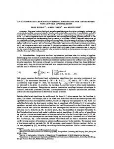
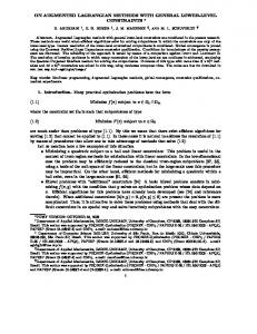
We define the level set of the distribution function of Y :  m Zp = y ∈ R : Pr[Y ≤ y] ≥ p . The set Zp is nonempty and closed for every p ∈ (0, 1) due to the monotonicity and the right continuity of the distribution function. Furthermore, its convex hull coZp is closed as well. Let p ∈ (0, 1]. A point v ∈ Rm is called a p-efficient point of the probability distribution function FY , if FY (v) ≥ p and there is no y ≤ v, y 6= v such that FY (y) ≥ p. Let p ∈ (0, 1) and let v j , j ∈ J, be all p-efficient points of Y , where J is an arbitrary set. We define the cones:SKj = vj + Rm + , j ∈ J. We have that Zp = j∈J Kj .  Pm+1 j m. i The convex hull is: coZp = α v : α ∈ S , j ∈ J + R m+1 i + i=1 i

Let f : Rn → R and gi : Rn → R, i = 1, . . . , m , and let D ⊂ Rn be a closed convex set.

The dual functional has the form ϕ(u) = inf L(x, z, u) = h(u) + d(u). D∗ = sup ϕ(u)

We analyze problem (P) under two sets of assumptions: Figure 1: Examples of the set Zp. Our problem can be compactly rewritten as follows:

• the function f is convex and the mapping g is concave, f and g are possibly non-smooth;

Optimality Conditions: Convex Problems

The Progressive Augmented Lagrangian

Constraint Qualification: x0 ∈ D and z 0 ∈ co Zp such that g(x0) > z 0. u ≥ 0 is an optimal solution if and only if there exists x ∈ X(u), points v 1, . . . , v m+1 ∈ V (u) and Pm+1 scalars β1 . . . , βm+1 ≥ 0 with j=1 βj = 1, such that

Step 0: Select a vector u1 ≥ 0 and solve the problems h(u1), d(u1). Let x1 and v 1 be the solutions. Set k = 1, ϕ(u1) = h(u1) + d(u1). Step 1: Ifϕ(uk ) ≥ (1 − γ)ϕ(w k−1) + γψ k−1(uk ), then w k = uk ; otherwise w k = w k−1. Step 2: Solve the master problem and denote by (xk , λk ) its solution.

j=1

L(x, z, u) = f (x) − hu, g(x)i + hu, zi.

∗ =D ∗≤P ∗ Pco

min f (x) subject to: g(x) ∈ Zp, x ∈ D.

βj v j − g(x) ∈ NRm+ (u)

Convex hull Problem: (Pco) min{f (x)|g(x) ≥ z, x ∈ D, z ∈ coZp}. Lagrangian function:

u≥0

where p is the probability level.

m+1 X

(P ) min f (x) subject to: g(x) ≥ z, x ∈ D, z ∈ Zp .

Dual problem: (D)

We consider the nonlinear programming problem min f (x) subject to Pr(g(x) ≥ Y ) ≥ p, x ∈ D.

We split variables to obtain the following problem formulation:

• the mappings f and g are twice continuously differentiable, f and g are possible nonconvex, resp. non-concave.

2 m  X 1 ̺X wik  j − kw k k2 λj vi − gi(x) + max 0, min f (x) + x,λ 2 i=1 ̺ 2̺ 

j∈Jk

x ∈ D, λ ∈ Sk .

Optimality Conditions: Smooth Problems

g(ˆ x) = wˆ + yˆ, I0(ˆ x) = {1 ≤ i ≤ m : yˆi = 0}. Constraint Qualification: There exists a feasible direction δ and a convex combination of pefficient points w such that ∀i ∈ I0(ˆ x) gi(ˆ x) + h∇gi(ˆ x), δi > w. First Order Necessary Condition of Optimality Lagrangian function: L(x, u) = f (x) − hu, g(x)i. Assume xˆ is an optimal solution of (1) and that condition C.Q is satisfied at xˆ. Then a vector uˆ ∈ Rm + exists such that −∇xL(ˆ x, uˆ) ∈ ND (ˆ x), − uˆ ∈ NcoZp (g(ˆ x)) Second Order Suficient Condition Y has a discrete distribution on a grid, D is polyhedral, xˆ satisfies FONCO, Λ(ˆ x) is the set of Lagrange multipliers FONCO. Theorem SOSC: ∀δ ∈ TD (ˆ x) such that gi(ˆ x) + h∇gi(ˆ x), βδi ≥ wi for all i ∈ I0(ˆ x), some convex combination of p-efficient points w, and β > 0 and h∇f (ˆ x), δi = 0, we have sup u∈Λ(ˆ x)

then xˆ is a minimum of (P).

x, u)δi hδ, ∇2xL(ˆ

> 0,

P P j j k Step 3: If gi(x ) ≥ j∈Jk λj vi − ε for all i = 1, . . . m and j∈Jk λj vi − gi(x) ≤ ε for all wik such that wik > ε, then stop; otherwise go to Step 4. Step 4: Calculate 
X j λj vi − gi(xk ) = max 0, wik + ̺ uk+1 i

Convergence

j∈Jk

Step 5: Find a p-efficient point v k+1 solution of d(uk+1). Step 6: Calculate dk+1(uk+1) = min huk+1, v j i,

h(uk+1) = f (xk ) + huk+1, g(xk )i,

j∈Jk+1 k+1

ϕ(uk+1) = h(u

The sequence of points w k generated by PAL converges to a solution of problem (Pco). The sequence ψ k (uk+1) converges to the optimal value D∗.

) + dJk+1 (uk+1),

ψ k (uk+1) = h(uk+1) + dJk+1 (uk+1)

References

Step 7. Set k → k + 1 by one, and go to Step 1.

Numerical Example: Supply Chain Problem X

min

fkm(xkm)

k∈K,m∈M

s.t: Pr[

X

xkm ≥ Ym, m ∈ M ] ≥ p,

k∈K X xkm ≤ Ck , xkm ≤ Bkkm, x ≥ 0.

m∈M

[1 ] Darinka Dentcheva, Gabriela Mart´ınez. Regularization Methods for Optimization Problems with Probabilistic Constraints. Submitted for publication. [2 ] Darinka Dentcheva, Gabriela Mart´ınez.Augmented Lagrangian Method for Probabilistic Optimization. Accepted in Annals of Operation Research.