Article
An Automated Approach for Mapping Persistent Ice and Snow Cover over High Latitude Regions David J. Selkowitz 1,2, * and Richard R. Forster 2 Received: 30 June 2015; Accepted: 21 December 2015; Published: 25 December 2015 Academic Editors: Daniel J. Hayes, Santonu Goswami, Guido Grosse, Benjamin Jones, Richard Gloaguen and Prasad S. Thenkabail 1 2
*
U.S. Geological Survey, Alaska Science Center, 4210 University Drive, Anchorage, AK 99508, USA Department of Geography, University of Utah, 260 S. Central Campus Dr., Room 270, Salt Lake City, UT 84112, USA;
[email protected] Correspondence:
[email protected]; Tel.: +1-907-786-7146; Fax: +1-907-786-7020
Abstract: We developed an automated approach for mapping persistent ice and snow cover (glaciers and perennial snowfields) from Landsat TM and ETM+ data across a variety of topography, glacier types, and climatic conditions at high latitudes (above ~65˝ N). Our approach exploits all available Landsat scenes acquired during the late summer (1 August–15 September) over a multi-year period and employs an automated cloud masking algorithm optimized for snow and ice covered mountainous environments. Pixels from individual Landsat scenes were classified as snow/ice covered or snow/ice free based on the Normalized Difference Snow Index (NDSI), and pixels consistently identified as snow/ice covered over a five-year period were classified as persistent ice and snow cover. The same NDSI and ratio of snow/ice-covered days to total days thresholds applied consistently across eight study regions resulted in persistent ice and snow cover maps that agreed closely in most areas with glacier area mapped for the Randolph Glacier Inventory (RGI), with a mean accuracy (agreement with the RGI) of 0.96, a mean precision (user’s accuracy of the snow/ice cover class) of 0.92, a mean recall (producer’s accuracy of the snow/ice cover class) of 0.86, and a mean F-score (a measure that considers both precision and recall) of 0.88. We also compared results from our approach to glacier area mapped from high spatial resolution imagery at four study regions and found similar results. Accuracy was lowest in regions with substantial areas of debris-covered glacier ice, suggesting that manual editing would still be required in these regions to achieve reasonable results. The similarity of our results to those from the RGI as well as glacier area mapped from high spatial resolution imagery suggests it should be possible to apply this approach across large regions to produce updated 30-m resolution maps of persistent ice and snow cover. In the short term, automated PISC maps can be used to rapidly identify areas where substantial changes in glacier area have occurred since the most recent conventional glacier inventories, highlighting areas where updated inventories are most urgently needed. From a longer term perspective, the automated production of PISC maps represents an important step toward fully automated glacier extent monitoring using Landsat or similar sensors. Keywords: remote sensing of glaciers; snow and ice; Landsat; arctic
1. Introduction Glaciers have been identified as one of the most sensitive indicators of changes in climate [1,2] and have been identified as an essential climate variable that should be monitored globally [3]. Glaciers not only respond to changes in climate, but can also drive changes in the earth climate system through changes in albedo and contribution to sea level rise [4–7]. From a more local to regional
Remote Sens. 2016, 8, 16; doi:10.3390/rs8010016
www.mdpi.com/journal/remotesensing
Remote Sens. 2016, 8, 16
2 of 21
perspective, glaciers often serve as a crucial source of runoff for downstream populations [8] and can present a potential hazard due to glacier lake outburst floods [9,10]. While the presence of exposed ice at the end of the melt season allows most glaciers to be positively identified under the right conditions, smaller glaciers cannot always be reliably distinguished from perennial snow cover patches. The challenge of discriminating between perennial snow cover patches and glaciers is confounded by the lack of satellite imagery acquired under ideal conditions when the maximum amount of ice is exposed. Consequently, even high quality glacier inventories created by image analysts may include some large perennial snow cover patches or omit some small glaciers. Image analysts are able to use contextual information (such as topographic position, patch shape, or ice or snow texture) to assist in discriminating between perennial snow cover patches and glaciers. Here we present a relatively simple automated approach designed to map glaciers that is likely to include a larger amount of perennial and consistently late lying seasonal snow cover patches than would be included in more traditional approaches. Therefore, although our intent is ultimately to map glaciers, we refer to the automated maps produced by the approach we describe as persistent ice and snow cover (PISC) maps, acknowledging that some perennial snow cover and late lying seasonal snow cover may be included. Despite the important role of glaciers in the global earth system, in situ monitoring efforts are limited to a tiny fraction of the areas containing glaciers [11]. While field measurements of mass balance are irreplaceable indicators of the status of specific glaciers, spaceborne remote sensing can provide crucial complementary information such as the areal extent of ice cover over large regions encompassing numerous glaciers. For this reason, remote sensing approaches have been implemented as a key component of the tiered global glacier monitoring strategy for the Global Terrestrial Network for Glaciers (GTN-G) [12]. Optical remote sensing using the visible through middle infrared bands has been the method of choice for the majority of remote sensing efforts attempting to map glaciers. This is due to both the widespread availability of optical remote sensing data from sensors such as those from the Landsat series and the Advanced Spaceborne Thermal Emission and Reflection Radiometer (ASTER) as well as the relatively unique spectral signature of snow and ice cover in the optical remote sensing wavelengths. Landsat image data have been used for a wide variety of glacier monitoring applications for more than 30 years. Early work with Landsat MultiSpectral Scanner (MSS) and Landsat Thematic Mapper (TM) focused on identification of glacier zones and calculation of corresponding reflectance values [13–18]. This was soon followed by glacier area mapping as well as change detection for areas covered by a single Landsat path-row [19–21]. Since the launch of the Landsat Enhanced Thematic Mapper Plus (ETM+) in 1999, numerous studies have used either the TM or ETM+ sensors (or in some cases, both sensors) to create glacier maps for increasingly large areas [22–26], with data from many of these studies included in the Global Land Ice Measurements from Space (GLIMS) database [27,28]. Even more recently, the Randolph Glacier Inventory (RGI) was compiled to be the first comprehensive glacier database with global coverage [29]. Despite the potential offered by remote sensing, comprehensive, fully inclusive glacier monitoring at spatial resolutions fine enough to detect changes in glacier area that typically occur over a decade or less has remained elusive in some regions. While global monitoring efforts such as GLIMS and more recently the RGI have been effective for mapping glaciers across many large regions, global coverage has only been achieved very recently and the glacier inventory dates within the global database span several decades. In addition, for many regions, mapping of changes in glacier area over time has not been conducted. One reason why such large area inventories have not been completed more regularly or for more regions is because existing approaches have required a substantial time investment by skilled image analysts. While previous work has demonstrated that automated classification results are typically as good or better than manually digitized results [30], even automated mapping approaches still require investment of an analyst’s time in the pre-processing stage (selection and acquisition of appropriate
Remote Sens. 2016, 8, 16
3 of 21
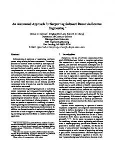
scenes with minimal cloud cover and minimal seasonal snow cover) as well as the post-processing stage (manual editing to correct classification errors, add areas of debris-covered glacier ice, and remove areas of perennial and seasonal snow cover, sea ice and icebergs) [31]. In many cases, input from an image analyst is also necessary to determine appropriate thresholds for band ratios or individual bands during the main processing stage. Manual correction of automatically-derived drainage divides from digital elevation models can also be a time consuming part of the process in some cases. We demonstrate that, across the circumpolar Arctic, and perhaps globally, the extent of PISC can be regularly monitored using fully automated processing of Landsat data that exploits all available cloud-free, shadow-free data available from the late summer period. This approach represents an important step toward fully automated monitoring of glacier extent across large regions. In addition, PISC maps generated by this approach can also be used to rapidly identify areas where substantial changes may have occurred since the most recent conventional glacier inventories were conducted and thus highlight areas where updated glacier inventories are most urgently needed. Finally, many applications can potentially benefit from regularly updated PISC maps, including land surface models, runoff models, and general circulation models (GCMs). 2. Study Regions We developed and tested the automated PISC mapping approach using data from four regions distributed throughout the Arctic, which we refer to as RGI calibration study areas (Figure 1, Table 1). Each RGI calibration study area covered a 35 ˆ 35 km area, with glaciers covering as much as 66% of the study domain at Bylot Island, Canada and as little as 11% of the study domain in the Brooks Range in the United States (as indicated by the RGI dataset). We tested the PISC mapping algorithm at four additional 35 ˆ 35 km study areas, referred to as RGI validation study areas, as well as at four smaller (approximately 15 ˆ 15 km) study areas where we acquired very high resolution imagery (VHRI) (Figure 1, Table 1), referred to as VHRI validation study areas. The selection of 35 ˆ 35 km bounding regions for the RGI calibration and RGI validation study areas was constrained to areas within the RGI database above 65˝ N with >5% ice cover where the dates of imagery used to construct the RGI glacier inventory were known to be within a single year. Allowing for these constraints, we selected 35 ˆ 35 km study areas to represent a range of glacier types, topography, and climatic conditions. The selection of VHRI validation study areas was constrained to areas above 65˝ N with >5% ice cover where acceptable very high resolution imagery from the period 2010–2015 was available from the DigitalGlobe archive of data from the WorldView 2 or WorldView 3 satellites (mention of a particular product does not constitute endorsement by the U.S. federal government). To be considered acceptable for our purposes, very high resolution imagery needed to contain a contiguous area of ~15 ˆ 15 km or larger with >5% ice cover that was cloud-free and nearly or completely free of late lying seasonal snow cover from the previous winter as well as nearly or completely free of recently accumulated snowfall. Allowing for these constraints, as with the selection of RGI calibration and RGI validation study areas, we selected study areas intended to represent a range of glacier types, topography, and climate conditions. Two of the four VHRI validation study areas were 15 ˆ 15 km in size, while the others were 16 ˆ 14 km and 17.5 ˆ 12.9 km due to cloud cover.
Remote Sens. 2016, 8, 16
4 of 21
Table 1. Study area locations and characteristics. Study Area
Country
Type
VHRI Sensor
Lat
Lon
Ice Cover
WRS-2 Path/Row
Brooks Range 1
USA
RGI calibration
n/a
69.3˝ N
144.0˝ W
11%
68/11, 69/12, 70/11, 71/11, 72/11
Saltfjellet
Norway
RGI calibration
n/a
66.7˝ N
14.2˝ E
26%
197/13, 198/13, 199/13, 200/13
RemoteBylot Sens.Island 2016, 8, 16 Canada
RGI calibration
n/a
73.4˝ N
79.0˝ W
66%
30/8, 31/8, 32/8, 33/8, 34/8, 35/8
RGI calibration RGI
n/a
71.8˝ N
25.0˝ W
61%
Jamesonland
Greenland
Clavering Greenland Island Clavering Greenland Island Barnes Ice Canada Cap Ice Cap Barnes Canada Trollaskagi Iceland Trollaskagi Peninsula Iceland Peninsula
Sarek NP
Sarek NP
Sweden
Sweden
Brooks Brooks 2 Range 2 Range Borden Borden Peninsula Peninsula
Canada Canada
Pond Inlet Pond Inlet
Canada Canada
USA
USA
Sverny Sverny Island Island
Russia Russia
validation RGI validation RGI RGI validation validation RGI RGI validation validation RGI RGI validation validation VHRI VHRI validation validation VHRI VHRI validation validation VHRI VHRI validation validation VHRI VHRI validation validation
n/a n/a
n/a n/a
n/a
n/a
n/a
n/a
WorldView 2
WorldView 2
74.3°N 74.3˝ N
69.6°N 69.6˝ N
65.7°N
65.7˝ N
67.3°N
67.3˝ N
69.2°N
69.2˝ N
21.0°W 21.0˝ W
72.0°W 72.0˝ W
18.8°W
18.8˝ W
17.7°E
17.7˝ E
144.8°W
144.8˝ W
20% 20%
47% 47%
8%
8%
10%
10%
6%
6%
226/9, 226/10, 227/9, 228/9, 231/9 227/8,229/9, 228/7,230/9, 228/8, 229/7,
230/7, 231/7 227/8, 228/7, 228/8, 229/7, 230/7, 231/7 22/11, 23/11, 24/11, 25/11 22/11, 23/11, 24/11, 25/11
218/14, 219/14, 220/14
218/14, 219/14, 220/14
196/13, 197/13, 198/13
196/13, 197/13, 198/13
69/11, 70/11, 71/11, 72/11
69/11, 70/11, 71/11, 72/11
WorldView ˝ WorldView 2 2 73.3˝73.3°N N 82.782.7°W W
47% 47%
33/8,34/8, 34/8, 35/8, 36/8 33/8, 35/8, 36/8
˝ WorldView WorldView 3 3 72.3˝72.3°N N 75.775.7°W W
83% 83%
27/9,28/9, 28/9, 29/9, 30/9 27/9, 29/9, 30/9
˝ WorldView WorldView 2 2 74.3˝74.3°N N 55.755.7°E E
34% 34%
177/8,178/7, 178/7, 178/8, 179/7, 177/8, 178/8, 179/7, 180/7 180/7
Figure Figure 1. Study Study area area locations locations across the circumpolar Arctic.
3. 3. Data Data Landsat Data 3.1. Landsat land areas areas on onthe thesurface surfaceofofthe theEarth Earthare areimaged imaged each active Landsat sensor every Most land byby each active Landsat sensor every 16 16 days, resulting in 22 or 23 potential scenes each year that cover a specific area of interest. For most days, resulting in 22 or 23 potential scenes each year that cover a specific area of interest. For conterminous United States, however, only only a limited selection of scenes regions outside outsideofofthe the conterminous United States, however, a limited selection of imaged scenes by the Landsat and ETM+ instruments have been downloaded archived [32], the imaged by theTM Landsat TM and ETM+ instruments have been and downloaded and resulting archivedin[32], availability faravailability less than 22–23 scenes for many [33]. Finally, persistent cloud cover resulting inofthe of far less per thanyear 22–23 scenesareas per year for many areas [33]. Finally, is an additional reduces the that number of useful surface views. of A useful typical surface glacier persistent cloud factor cover that is anfurther additional factor further reduces the number views. A typical glacier effort monitoring or identifying mapping effort involves identifying cloud-free images monitoring or mapping involves cloud-free images (or portions of images), or (or for portions of images), or offor largeracquired regions,during collection of images, acquired the seasonal larger regions, collection images, the seasonal minimum snowduring cover extent period. minimum snow cover extent period. While in theory this is straightforward, the typically short duration of the snow-free period on and around glaciers does not always coincide with the availability of a cloud-free satellite acquisition. As a result, accurate glacier mapping requires careful scene selection by skilled analysts with knowledge of the region and the seasonal snow cover conditions during the period of interest. The analyst must select optimal scenes for automated or
Remote Sens. 2016, 8, 16
5 of 21
While in theory this is straightforward, the typically short duration of the snow-free period on and around glaciers does not always coincide with the availability of a cloud-free satellite acquisition. As a result, accurate glacier mapping requires careful scene selection by skilled analysts with knowledge of the region and the seasonal snow cover conditions during the period of interest. The analyst must select optimal scenes for automated or semi-automated glacier classification [30]. Overlapping Landsat paths result in more frequent image acquisitions for locations covered by more than 1 path. While only about 5% of the land surface is covered by multiple paths at the equator [34], at high latitudes, due to the convergence of Landsat paths, path overlap is ubiquitous, with many ground locations covered by three or more Landsat paths. This results in a doubling or even tripling of the number of Landsat scenes covering an area of interest. Assuming a substantial portion of these scenes have been acquired and archived (global scene availability is described in [33]), the odds of finding one or more scenes (or portions thereof) that capture the minimum annual extent of snow and ice under cloud-free conditions theoretically increases substantially with latitude. In our approach, we exploit this relative abundance of scenes available at many high latitude locations and consider all available Landsat TM or ETM+ data for each location, using an automated cloud classification algorithm to identify all instances of cloud-free views for each pixel location. The majority of studies mapping glacier area using Landsat data have used uncorrected raw digital number (DN) or top-of-atmosphere (TOA) reflectance image data. Previous work has shown, however, that the use of atmospherically corrected surface reflectance image data can improve the accuracy of the results [35], and that atmospheric correction is particularly crucial if the Normalized Difference Snow Index (NDSI), which incorporates Landsat band 2 where atmospheric scattering is particularly high, is used [36]. To limit errors that could be introduced by variable atmospheric conditions when applying a standardized algorithm across large regions and over different dates, we make use of the atmospherically corrected USGS surface reflectance climate data record (CDR) product available for the Landsat TM and ETM+ sensors [37]. The surface reflectance CDR applies atmospheric correction routines originally developed for the Moderate Resolution Imaging Spectroradiometer (MODIS) to Landsat data. Surface reflectance is computed using the Second Simulation of a Satellite Signal in the Solar Spectrum (6S) radiative transfer model, which requires water vapor, ozone, geopotential height, aerosol optical thickness, and a digital elevation model along with Landsat TOA reflectance data. Application of 6S at high latitudes does violate the assumption of a plane-parallel atmosphere, which can impact the quality of surface reflectance product. However, because this is the standard atmospheric correction approach currently applied to all Landsat scenes and because we have not seen any evidence of errors large enough to affect the ability to discriminate between ice or snow and other surfaces in high latitude Landsat surface reflectance data, we have opted to use the standardized Landsat surface reflectance product. For the RGI calibration and RGI validation study areas, we acquired and processed Landsat top-of-atmosphere (TOA) reflectance and surface reflectance products [36] from all available Landsat TM and ETM+ scenes available during the late summer (in this case defined as 1 August–15 September) for five-year periods. The TOA and surface reflectance Landsat scene products were produced by and acquired from the USGS EROS Data Center. We used the EarthExplorer interface to identify scenes acquired during the time period of interest at each of our study areas and then submitted orders for the identified scenes, subset to our study areas, using the EROS Science Processing Architecture (ESPA) interface. For the RGI calibration and RGI validation study areas, scenes were acquired for the five-year period centered on the date of the RGI inventory. At the Saltfjellet, Norway primary study area we acquired data from an additional year (for a total of six years) due to the poor availability of cloud-free scenes over the five-year period centered on the RGI mapping year. For the VHRI validation study areas, we acquired Landsat scenes for the 2010–2014 period, as the very high resolution imagery was acquired during 2014 or 2015.
Remote Sens. 2016, 8, 16
6 of 21
3.2. Randolph Glacier Inventory Data At each of the four RGI calibration study areas, we used glacier polygons provided by the RGI (version 4.0) to conduct sensitivity analysis for two key thresholds described below, as well as to conduct an accuracy assessment of mapped glacier area using our automated approach. The RGI provides polygon datasets of all glaciers in a region mapped using a variety of image resources, including Landat TM and ETM+ data. While the imagery source and mapping approach are not identified in the RGI database, the date or range of dates used to map each glacier are included in the database for most entries. Although some RGI polygons indicate a range of years and others provide no information about date or year of the image or other resource used for mapping, all RGI data used in this study indicated a specific date or range of dates within a single year covering the entire extent of each 35 ˆ 35 km study area. Remote Sens. 2016, 8, 16 4. Methods
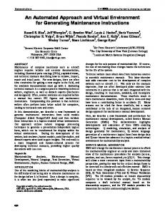
For4.each pixel in the study domain, our approach identifies the available cloud-free, shadow-free Methods (and otherwise valid) land surface views and then compiles a the stack of NDSI valuesshadow-free corresponding to For each pixel in the study domain, our approach identifies available cloud-free, each valid surface view. threshold is then applied to of the stack of NDSI values totoidentify (andland otherwise valid) landAsurface viewsvalue and then compiles a stack NDSI values corresponding each valid land is then applied theice-free. stack ofThe NDSI values to each land surface viewsurface in theview. stackAasthreshold snow orvalue ice-covered or snowtoor ratio of days with identify land surface viewwe in the stack or ice-covered or snow TheCover ratio of(fDISC) snow/ice to theeach total days, which refer to as as snow the fraction of Days withor Iceice-free. or Snow with snow/ice to the total days, which we refer to as the fraction of Days with Ice or Snow is then days computed and a second threshold value is used to identify the pixel as PISC or PISC-free. Cover (fDISC) is then computed and a second threshold value is used to identify the pixel as PISC or A diagram of this processing flow is presented in Figure 2. PISC-free. A diagram of this processing flow is presented in Figure 2.
Figure 2. Diagram of processing flow for classification of Persistent Ice and Snow Cover (PISC) for a
Figure 2. Diagram of processing flow for classification of Persistent Ice and Snow Cover (PISC) for single pixel. a single pixel. 4.1. Cloud and Shadow Masking Analysis of stacks of numerous Landsat scenes requires an accurate automated cloud-masking approach. The CFmask algorithm [38] uses a series of rules based on cloud physical properties to develop a potential cloud layer from Landsat top-of-atmosphere reflectance data in bands 1–5 and 7 as well as brightness temperature from band 6. The potential cloud layer is then segmented to produce cloud objects, and ultimately a cloud mask and cloud-shadow mask that is provided with
Remote Sens. 2016, 8, 16
7 of 21
4.1. Cloud and Shadow Masking Analysis of stacks of numerous Landsat scenes requires an accurate automated cloud-masking approach. The CFmask algorithm [38] uses a series of rules based on cloud physical properties to develop a potential cloud layer from Landsat top-of-atmosphere reflectance data in bands 1–5 and 7 as well as brightness temperature from band 6. The potential cloud layer is then segmented to produce cloud objects, and ultimately a cloud mask and cloud-shadow mask that is provided with each USGS Climate Data Record (CDR) Landsat surface reflectance scene. While the overall accuracy Remote 2016, 8, 16 of the Sens. CFmask cloud mask has been reported as 96.4%, our evaluation of CFmask cloud masks found that in rocky, alpine terrain and areas with a mixture of snow, ice, and other land cover types, the CFmask cover (an example is CFmask algorithm algorithm was was prone proneto toerrors errorsofofcommission commission(false (falsepositives) positives)for forcloud cloud cover (an example shown in in Figure importantly, is shown Figure3).3).More More importantly,the theerrors errorsofofcommission commissionwere were not not randomly randomly distributed distributed across areas with rock and ice cover, but were consistently present at the same patches of across areas with rock and ice cover, but were consistently present at the same patches of land land cover cover on multiple occasions, thus resulting in a potential bias in available cloud-free data. We considered on multiple occasions, thus resulting in a potential bias in available cloud-free data. We considered the the high high rate rate of of errors errors of of commission commission and and particularly particularly the the potential potential for for bias bias to to be be unacceptable unacceptable for for our purposes. We implemented a revised cloud masking approach designed to reduce errors our purposes. We implemented a revised cloud masking approach designed to reduce errors of of commission commission from from the the CFmask CFmask cloud cloud masks masks over over mountainous mountainous environments environments dominated dominated by by rock, rock, snow, and ice, ice, allowing allowing us us to to fully fully exploit exploit nearly snow, and nearly all all available available cloud-free cloud-free land land surface surface views views acquired acquired during the late summer period. The revised cloud masking approach employed classification trees during the late summer period. The revised cloud masking approach employed classification that all instances of pixels wherewhere the CFmask product indicated cloudcloud cover.cover. The trees reevaluated that reevaluated all instances of pixels the CFmask product indicated classification trees were originally developed for a seasonal snow covered area monitoring project The classification trees were originally developed for a seasonal snow covered area monitoring project and arebased basedon onover over 100,000 pixels acquired from 20 Landsat scenes from mountainous areas and are 100,000 pixels acquired from 20 Landsat scenes from mountainous areas across across the The globe. The classification tree approach reliesfrom on data from Landsat bands and 7 to the globe. classification tree approach relies on data Landsat bands 1–5 and 7 to1–5 make a final make a final distinction between cloud-covered and cloud-free pixels in cases where the original distinction between cloud-covered and cloud-free pixels in cases where the original CFmask indicated CFmask indicated Testing tree of the classification tree approach in original conjunction withdata the cloud cover. Testingcloud of thecover. classification approach in conjunction with the CFmask original indicated in a slight improvement in overall (from 89%improvement to 91%), within a indicatedCFmask a slightdata improvement overall accuracy (from 89% to accuracy 91%), with a major major improvement in accuracy for high mountain areas from around the globe with substantial accuracy for high mountain areas from around the globe with substantial snow and ice cover (from snow ice cover (from 66% to 88%). 66% toand 88%).
Figure 3. Comparison Figure 3. Comparison ofof original original CFmask CFmask and and revised revised CFmask CFmask for for Bylot Bylot Island Island Landsat Landsat scene scene acquired 12 August 1999. (a) Landsat surface reflectance 7-4-2 band combination; (b) CFmask original acquired 12 August 1999. (a) Landsat surface reflectance 7-4-2 band combination; (b) original CFmask cloud cover classification; and (c)CFmask revised cloud CFmask cloud cover classification. cloud cover classification; and (c) revised cover classification.
In addition to cloud cover, both cloud shadows and terrain shadows can impact surface In addition to cloud cover, both cloud shadows and terrain shadows can impact surface reflectance to the extent that band ratios such as the NDSI no longer provide a reliable indication of reflectance to the extent that band ratios such as the NDSI no longer provide a reliable indication land surface characteristics. We excluded the most deeply shadowed pixels from further analysis by masking pixels where apparent surface reflectance in both bands 2 and 4 was