nor does it imply that those items are necessarily the best available. ... Although our toolset offers performance measurement and visualization, it does so .... simplifies the interaction between the visualization module and our database hosting.
An Automated Benchmarking Toolset1 Michel Courson2, Alan Mink, Guillaume Marçais3, Benjamin Traverse3 100 Bureau Drive, Stop 8951 Gaithersburg MD 20899-8951, USA {michel.courson, amink, guillaume.marcais}@nist.gov
Abstract. The drive for performance in parallel computing and the need to evaluate platform upgrades or replacements are major reasons frequent running of benchmark codes has become commonplace for application and platform evaluation and tuning. NIST is developing a prototype for an automated benchmarking toolset to reduce the manual effort in running and analyzing the results of such benchmarks. Our toolset consists of three main modules. A Data Collection and Storage module handles the collection of performance data and implements a central repository for such data. Another module provides an integrated mechanism to analyze and visualize the data stored in the repository. An Experiment Control Module assists the user in designing and executing experiments. To reduce the development effort this toolset is built around existing tools and is designed to be easily extensible to support other tools. Keywords. Cluster computing, data collection, database, performance measurement, performance analysis, queuing system, visualization.
1. Introduction The drive for performance in parallel computing and the need to evaluate platform upgrades or replacements are major reasons frequent running of benchmark codes has become commonplace. By “benchmark code” we refer not only to well known codes designed to evaluate platforms, but also to any piece of code used for performance evaluation or in need of tuning. NIST is developing a prototype of an automated benchmarking toolset to reduce the manual effort involved in running benchmarks, to provide a central repository for all the collected data, current and archival, and to provide an integrated mechanism to analyze and visualize that data. To reduce the development effort and leverage the work of other tool developers, we intend to build this benchmarking toolset around existing tools and only produce “glue” and “gap” code as necessary. Such an automated benchmarking toolset will support both production environments and research environments. For a production environment such a toolset 1
This NIST contribution is not subject to copyright in the United States. Certain commercial items may be identified but that does not imply recommendation or endorsement by NIST, nor does it imply that those items are necessarily the best available. 2 Visiting scientist from University of Maryland, UMIACS. 3 Guest researcher from the Institut National des Télécommunications, France.
can reduce the manual effort required and speed up the overall benchmark and evaluation process. In addition, the database will provide a means to produce unplanned comparisons over a much longer epoch, limited by the age of the database. Through its database of performance information, such a toolset also provides a rich environment for standard and innovative performance analysis, as well as a means to produce unplanned comparisons. Automated Benchmarking Tool 1. Data Collection and Storage
2. Analysis and Visualization
3. Experiment Design and Control
Data Description
Visualization
Experiment Specification
Data Collection
Data Analysis
Experimental Plan Design
Storage
Cluster Metrics Exploratory techniques
Run Control Front End
Statistics
Fig. 1. Project Organization Chart
1.1 Design Overview The proposed benchmarking toolset consists of three major modules as shown in Figure 1: (1) the Data Collection and Storage module, (2) the Analysis and Visualization module, and (3) the Experiment Design and Control module. The Data Collection and Storage module addresses the runtime collection and storage of performance data for later retrieval. The data storage organization is based on an abstract model of our computing prototype environment, a computing cluster of PCs. This abstract model is mapped on a regular SQL database. We use the PostgreSQL [POS] database management package. The collection of data is done with the SNMP protocol, using the Scotty package [TNM]. However, the tool is general enough to handle virtually any other packages implementing the SQL and SNMP protocols. The Analysis and Visualization module provides the means to produce standard plots and charts of the raw data from the database or composite values using well known tools such as MatLab [MAT] or IDL [IDL]. This module is intended to be user extensible to allow novel and innovative techniques such as data mining to identify hidden patterns in the data. The Experiment Design and Control module automates the definition and execution of a set of experiments. This is accomplished from a combination of information supplied by the experimenter and information extracted from the database. The culmination of this module is the execution of a set of run-time scripts; these carry out the benchmark code executions and subsequent data collection and storage of the associated performance data. Each component is built modularly using existing open software for more flexibility and may be easily modified for experimentation with alternate features and capabilities.
1.2 Existing Work Many tools have been developed that focus on performance measurement. Some of the most well known include: VAMPIR [VAM99], from the German company Pallas GmbH, for MPI programs, AIMS [YAN96] from NASA Ames Research Center, Paradyn [MIL95] that features performance tracing down to the statement level through dynamic instrumentation, and Pablo [AYD96] which is known for its visualization and self-defining format, among other features. These tools focus much more extensively than our toolset on instrumenting codes to collect and compute performance measurement metrics and on locating computational bottlenecks. These and other tools also provide various visualization capabilities. Although our toolset offers performance measurement and visualization, it does so by incorporating other existing tools, possibly some of the tools mentioned above. In addition our toolset focuses on an integrated database that spans all the “benchmark” codes over an extended time frame. This differs from current effort of the Paradyn team [MIL99], which tracks the performance of a single code with the intention of better tuning of that code. Our toolset will also provide the capability to design and manage the evolution of experiments consisting of multiple codes as well as their input and output files.
2. Performance Data Model This section describes an abstract data model of a parallel computing environment that represents the performance data available from our cluster in a compact but accurate fashion. To implement this model, we selected a set of collection mechanisms and tools as well as a storage platform using a relational database. 2.1. Performance Data Storage Platform We designed a formal data model to represent both abstract data structures, mechanisms and relationships within the data. This model is described in detail on our website. Although specifically designed to represent a computing cluster, this abstract model is easily changeable for other platforms. The data stored in the database is a set of “snapshots” (runs). The key feature of the model lies in the ability to create virtual experiments: such experiments are conducted without actually running the application, but by combining instead existing runs from previous experiments, promoting reuse of existing performance data. Although an object-oriented database management system (OODBMS) may seem best suited for our data model, we did not find any OODBMS that meets our requirements for convenient querying and easy retrieval for the user. Such features are readily available from most database management systems supporting SQL, at the cost of a little extra administration overhead. The actual database is implemented using PostgreSQL [POS], a freely available SQL relational database. The entity-relationship diagram (fig. 2) translates to a set of corresponding tables. Each table is the representation of an entity type; each column represents attributes,
each row is one occurrence. Primary keys (unique identifiers) are used to ensure uniqueness and to allow cross-references between tables. As noted before, this makes the database administration less straightforward due to complex key management. However this complexity is only a burden for the tool administrator, not the user. Our reference database implements most of the model and provides two other interesting features. First of all, it supports time series using a variable-granularity scheme similar to Paradyn [MIL95]; common statistics such as average are also cached in the database to facilitate simple queries. Our toolkit also provides a generic registry mechanism to store information without administrator privileges to create new tables, for example application-specific tracing information.
EXPERIMENT n
1 n RUN
1
VIRTUAL MACHINE 1
1 n NETWORK DEVICE
n MACHINE
1 n DEVICE TIME SERIES
1 1 GPS DEVICE
1
n
1
PROCESS 1
1 MULTIKRON DEVICE
n PROCESS TIME SERIES
Fig. 2. Entity-Relation Diagram
2.2 Collection Tools The automated benchmarking toolset is designed to handle data collection from most sources. In order to demonstrate the collection mechanism, our reference implementation currently supports several mechanisms at different levels in the parallel machine, as described below. For low-level data such as memory usage, paging activity or network usage at the process level, we use a modified version of UCD-SNMP [UCD], a popular, freely available, easily extensible SNMP agent from the UC Davis. The agent already supports a very wide range of system-level data such as network activity, via standard interfaces. It was extended to give fast access to common statistics such as load average, process activity and resource usage, as well as our custom high-resolution tracing hardware, Multikron [MIN95], and GPS-synchronized timing facility. This information is collected and stored as time-series data. Application-level data such as response time or number of processors is collected directly from the run control module (see below).
Our toolset is designed to support most third-party measurement tools that follow our data model. We have demonstrated this by collecting high-level performance data from the MPI Profiling library developed at NIST [IND99]. This library provides transparent timing and call-count information for most MPI functions (send, receive, etc.) as well as synthetic metrics including computation, communication and response time for any MPI application.
3. Experiment Design and Control The Experiment Design and Control module provides a means to quickly and efficiently design and carry out experiments. The experiment design is shown in Figure 3. The user specifies the desired parameters that will control the execution of the application and their different values. The tool then builds an experimental plan that will analyze these parameters in an efficient way, relying on advanced statistical techniques as well as existing runs in the database to minimize the overall cost of the experiment (both in terms of time and resources). The Run Module then automatically carries out the experimental plan by executing the necessary program instantiations. E xperi men t D esign Su b mo du le Experiment Sp ecif ica tio n
Ch eck Re triev e Info rm ation Sto re
Data Ba se
Plan plug-in
Experimental Plan D es ign
Plan plug-in
Test Plan plug-in
Re triev e Param eters
Store R un C on trol Su bmo du le Ru n Packa ge M pipro file
Collec tion Packa ge
SNM P Add-o n
Fig. 3. Experiment Control and Design Module
3.1 Experiment Specification We define an experiment by a set of variables (e.g. application, number of processors, etc.) and a set of values they can take. This mechanism is general enough to describe most any situation the experimenter may want to describe. Our tool provides a graphical interface that guides the experimenter through the experiment specification process. Figure 4 illustrates some of the steps followed to define the experiment. First the user selects the set of applications he wishes to study. For each application, he defines a set of variables that will control the execution of the experiment, such as the number of processors or the input file. For each variable, the user declares a set of values that these variables can take during the experiments, for example a range of 2 to 16 for a scalabilty test or different communication libraries. At each step the tool interacts with the database to propose choices from previous runs. The sample experiment shown below simultaneously tests the scalability of two applications as well as their performance using different communication libraries.
Fig. 4. Screenshots of the Experiment Design Submodule
3.2. Experimental Plan Design An experimental plan describes the way an experiment should be carried out. The simplest case is a set of fully described runs, that is, an instance of each application run with each combination of the controlling variables' specified values declared in the experiment. Designing such an experimental plan follows a well-known process [BOX78], widely used in most scientific disciplines. Based on the requirements (e.g. standard error, interactions), such techniques define the optimal set of runs that match the requirements at the lowest cost (in terms of time and resources). A number of plan-design plug-ins can drive this package. Our initial prototype provides fulln factorial plans, that select all the possible combinations of the variables (O(e )), but we expect future support of fractional-factorial plans (up to O(n) with no interactions). The next step consists of storing the fully described experiment in the database as an experiment structure pointing to a list of runs. If some of the runs needed for the experiment already exist in the database, they can be reused to save time if the experimenter desires; records for the missing instances are created in the database and flagged for execution by the Run Package. A graphical interface helps the user through the selection of existing runs, providing the choice to hand-pick them, to let the system chose one or to forcibly re-execute the application. 3.3. Run Control The Run Package, as shown in Figure 3, establishes the link between the previously described collection tools and the database. The run package carries out the individual executions (runs) required in the experiment and manages the performance data collection process. This component is fully automated. It relies on an existing queuing system for most of the job control. Our prototype uses DQS [DQS], a free, open-source job control system from the Florida State University. As with most queuing systems, a job is submitted in the form of a single shell script containing special control directives. For a given experiment, it accesses the database and retrieves the list of runs to be executed. One of the variables stored in the database has a special meaning: it points to a command file for the job control system, provided by the user as a template for the tool. For each run, the run package builds a new job by parsing the command file for variable substitution and instrumenting it with data collection commands. The created jobs are then submitted in a single batch to the job control system for execution. The instrumentation code within the job file is responsible for starting and stopping the collection tools as well as updating the records in the database once the job is completed.
4. Visualization and Analysis The toolset provides an extensible visualization and analysis package. This package initially offers basic capabilities to visualize the performance data collected
as well as to perform standard statistical analysis. We also devised several computed metrics adapted to get insight of performance issues specific to parallel computing architectures. As with the rest of the toolkit, it can be easily extended to support new analysis techniques, for example data mining. 4.1 Visualization tools The requirements for our visualization module are the capability to plot any pair of raw data items from the database (e.g. memory usage against time), the capability to display graphical tests and finally the capability to plot values from computed metrics. The visualization tool is built on top of a third-party software package. We have chosen to use MatLab [MAT] or IDL [IDL] software, which are commercial software. They both offer good drawing capabilities in 2D and 3D. Moreover, they are able to conduct standard statistical analysis and to perform fast array/matrix computation. Both of the tools can access a database using the ODBC protocol. This feature simplifies the interaction between the visualization module and our database hosting the experiments’ performance results. Finally, these two pieces of software are available for the Win95/98/NT platform, MacOS and many UNIX platforms. This allows our toolset's visualization package to run on many platforms and not only UNIX, our primary development system. The use of free software such as Octave [OCT] rather than commercial software is also possible. It offers the same basic interface, computation and drawing capabilities as MatLab, but it has no database connectivity embedded and is only available for Win95/98/NT and UNIX.
4.2 Analysis The analysis package helps to interpret the meaning of the performance data and get some insight into the application and/or parallel machine behavior. It uses an integrated visualization tool (see above) as a graphical output and computing platforms as needed. It will assist in performing essential statistical analysis such as standard deviation, standard error, etc. It will also provide a set of less common graphical tests to validate the results of the experiment: independence between runs, fixed location of measurements, etc. We also developed a suite of new metrics focusing on different aspects specific to cluster computing, summarized in Table 1. These metrics rely on a simple "Communication v. Computation" model. Although this model has its limitations (it cannot describe particular cases, such as superlinear speed up), it is rich enough to help understand the internal behavior of parallel codes. These metrics are all computed from high-level runtime computation and communication information. Each one focuses on a different aspect of the execution of a parallel job. We use the standard speedup (SU) and the efficiency (EF) as general indicators of the gain in speed. We define several overhead metrics: the global overhead (GOH) as the overhead introduced in the process of parallelizing the code compared to the sequential version and the computation overhead (POH) as the extra computation cost alone. We also define the average response time on the parallel
program, which gives an indication of the load balancing, the granularity (computation-communication ratio) and the mean number of working processors. This set of metrics helps in determining what can be modified in the program or the architecture to improve performance. The analysis package will feature an automatic diagnostic of the application using such metrics to pinpoint potential improvements. We present this set of metrics as a basis to demonstrate the functionality of the module. The user can extend the toolset with other analysis schemes and techniques to highlight particular points of parallel programs. Definition
R SU = s Rp SU n
EF =
å =
n
Rp
i =1
GOH =
Ri
n n R p − Rs Rs
å POH =
n
P − Rs
i =1 i
Description Speedup.
Efficiency. Average response time of the parallel version.
Global Overhead: overhead of parallel section of the code compared to the sequential version. Computation Overhead: part of the global overhead due only to computational operations.
Rs
å η= å
n
Xi
i =1 n
Granularity: Communication vs. Computation ratio.
P
i =1 i
n=
1 Rp
å
n
P i =1 i
Xi: Communication time; Pi: Computation time;
Mean number of working processors
Ri=Xi+Pi: response time of i-th process out of n Rs: response time of the sequential version Table 1. Parallel Metrics
5. Summary and Conclusions Our automated benchmarking toolset is intended to provide an extensible environment for conducting traditional computing platform evaluations as well as research-based computer/application performance analysis. The key mechanism is a central database that incorporates an abstract model of the computing platform. The
database stores all available runtime performance and configuration information for each execution of each program and provides current and archival information for analysis and visualization. Various existing tools, covering such functions as data collection, analysis, visualization and runtime control, will be integrated with this database. Our goal is to integrate any performance, visualization or analysis tool into this toolset, treating these modules as interchangeable "plug-ins." To accomplish this we need a methodology to access these various possible disjoint tools. One possible approach would be to specify an access API to these tools that would activate commands or processes and exchange information. Our initial prototype already incorporates an SQL-based database along with SNMP data collection from the various data agents on the executing platforms. We are using Tcl/Tk to handle most of the integration between the various tools and for the user interface. We are currently working on the Experiment Control Package, the access APIs and a front-end to bind the different components into a single tool. Additional information, downloads and current status of this project is available on our website at http://www.cluster.nist.gov.
References [AYD96] Ruth A. Aydt, “The Pablo Self-Defining Data Format”,http://www.pablo.cs.uiuc.edu. [BOX78] George E.P. Box, William G. Hunter, “Statistics for Experimenters, an introduction to design, data analysis, and modeling building”, 1978. [DQS] “DQS - Distributed Queueing System”, http://www.scri.fsu.edu/~pasko/dqs.html [IDL] “IDL - The Interactive Data Language”, http://www.rsinc.com/idl/index.cfm [IND99] "MPIProf", http://www.itl.nist.gov/div895/cmr/mpiprof [MAT] “The MathWorks - MATLAB Introduction”. http://www.mathworks.com [MIL95] B.P. Mille et al., “The Paradyn Parallel Performance Measurement Tools”, IEEE Computer, 28, 1995. [MIL99] Barton P. Miller, Karen L. Karavanic. “Improving Online Performance Diagnosis by the Use of Historical Performance Data”, SC'99, Portland, Oregon (USA) November 1999. [MIN95] Alan Mink, “The Multikron Project", http://www.multikron.nist.gov [OCT] “Octave Home Page”, http://www.che.wisc.edu/octave [POS] “PostgreSQL Home Page”, http://www.pyrenet.fr/postgresql [TNM] “Scotty - Tcl Extensions for Network Management”, http://wwwhome.cs.utwente.nl/~schoenw/scotty [UCD] University of California at Davis, “The UCD-SNMP project home page”, http://www.ece.ucdavis.edu/ucd-snmp [VAM99] Pallas Gmbh, “VAMPIR”, http://www.pallas.de/pages/vampir.htm, 1999. [YAN96] J. C. Yan and S. R. Sarukkai, “Analyzing Parallel Program Performance Using Normalized Performance Indices and Trace Transformation Techniques”, Parallel Computing Vol. 22, No. 9, November 1996. pages 1215-1237, 1996.