In a clinical setting, it may be difficult for a doctor on-call or a radiologist ... 1 The SBD data sets were provided by the Brain Imaging Centre, Montreal Neurolog-.
An Automated Multi-spectral MRI Segmentation Algorithm Using Approximate Reducts ´ ezak3,1 Sebastian Widz1 , Kenneth Revett2 , Dominik Sl¸ 1
3
Polish-Japanese Institute of Information Technology, Warsaw, Poland 2 University of Luton, Luton, UK Department of Computer Science, University of Regina, Regina, Canada
Abstract. We introduce an automated multi-spectral MRI segmentation technique based on approximate reducts derived from the data mining paradigm of the theory of rough sets. We utilized the T1, T2 and PD MRI images from the Simulated Brain Database as a ”gold standard” to train and test our segmentation algorithm. The results suggest that approximate reducts, used alone or in combination with other classification methods, may provide a novel and efficient approach to the segmentation of volumetric MRI data sets. Keywords: MRI segmentation, approximate reducts, genetic algorithms
1
Introduction
In Magnetic Resonance Imaging (MRI) data, segmentation in a 2D context entails assigning labels to pixels (or more properly voxels), where the labels correspond to primary parenchymal tissue types: usually white matter (WM), gray matter (GM), and cerebral spinal fluid (CSF). It has been demonstrated repeatedly that the relative distributions of and/or changes in the levels of primary brain tissue classes are diagnostic for specific diseases such as stroke, Alzheimer’s disease, various forms of dementia, and multiple sclerosis to name a few [3, 4]. Segmentation process is usually performed by an expert who visually inspects a series of MRI films. In a clinical setting, it may be difficult for a doctor on-call or a radiologist to have sufficient time and/or the requisite experience to analyze the potentially voluminous and variable nature of MRI that is produced in a busy hospital setting. Therefore, any tool which provides detailed and accurate information regarding MRI analysis in an automated manner may be valuable. The segmentation accuracy is estimated as a similarity measure between the results of the algorithm and the expert’s evaluation. Therefore, a kind of ”gold standard” – an objective and verifiable MRI data set where every voxel is classified with respect to tissue class with 100% accuracy, is helpful. One such gold standard is the Simulated Brain Database (SBD) 1 . It contains a series of 1
The SBD data sets were provided by the Brain Imaging Centre, Montreal Neurological Institute (http://www.bic.mni.mcgill.ca/brainweb).
3D volumetric multi-spectral MRI data sets (T1, T2, PD) with axial orientation. Every set consists of 181 slices (1mm slice thickness), where each slice is 181∗217 voxels, with no inter-slice gaps. A number of different data sets are available with varying with slice thickness, noise ratios and field inhomogeneity (INU) levels which can be set to the user defined values. SBD provides an opportunity to investigate segmentation algorithms in a supervised manner. One can generate a classification system using the classified volume for training and then test on volumes not included in the training set. Traditionally, MRI segmentation methods have been performed using cluster analysis, histogram extraction, and neural networks [1, 5, 7, 15]. In this paper, we present an approach based on the concept of approximate reducts [10–12] derived from the data mining paradigm of the theory of rough sets [6, 9]. We utilize T1, T2, and PD MRI modalities from SBD for training and testing. Decision tables are generated as basing on the set of 10 attributes extracted from the training volumes (1mm horizontal slices) where the classification is known. Using an order based genetic algorithm (o-GA) (cf. [2, 14]), we search through the decision table for approximate reducts resulting in the simple ”if..then..” decision rules. After training, we test the rule sets for segmentation accuracy across all imaging modalities along three variables: slice thickness, noise level and intensity of inhomogeneity (INU). The segmentation accuracy varies from 95% (T1, 1mm slices, 3% noise, and 20 % INU) to 75% (PD, 9 mm, 9% noise, and 40% INU) using training set 1mm 3preprocessing, these data agree favorably with more traditional and complicated approaches. It suggests that approximate reducts may provide a novel approach to MRI segmentation. The article is organized as follows: In section 2, we describe the data preparation technique, which involves attribute selection and quantification. In section 3, we describe the algorithms employed to find approximate reducts and decision rules used in the testing phase of the segmentation process. Next we present the results of this analysis in section 4 and a brief discussion follows in section 5.
2
Data Preparation
In the rough set theory the sample of data takes the form of an information system A = (U, A), where each attribute a ∈ A is a function a : U → Va from the universe U into the value set Va . In our case the elements of U are voxels taken from MR images. There are 181 ∗ 217 ∗ k objects, where k denotes the number of MRI slices for a specified thickness. The set A contains the attributes labelling the voxels with respect to the MRI modalities illustrated in Figure 2. The goal of MRI segmentation is to classify voxels into their correct tissue classes using the available attributes A. We trained the classifier using a decision table A = (U, A ∪ {d}), where the additional decision attribute d ∈ / A represents the ground truth. We can consider five basic decision classes corresponding to the following types: background, bone, white matter (WM), gray matter (GM), and cerebral spinal fluid (CSF) (cf. Figure 1). In our approach we restrict our classification algorithm to WM, GM, and CSF voxels. Below we characterize the method we employed to extract the attributes in A from the MRI images.
Magnitude: Magnitude attributes, denoted by magT 1 , magT 2 , magP D , have the values derived from frequency histograms for T1, T2, and PD modalities. Figure 1 below graphically displays the total voxel content of a single SBD T1-weighted slice. There are several peaks which can be resolved using standard polynomial interpolation techniques. We used a set of Matlab Polynomial Toolbox functions (Polyfit and Polyval) and normalized the y-axis to smooth out the histogram in order to find the peaks. We extracted the Full-Width Half-Maximum (FWHM) interval for each peak (which is approximately centered about the mean). We labelled the objects-voxels belonging to each such FWHM with specific values of magT 1 in our decision table. In the same way, we labelled the objects belonging to the gaps between those intervals with some intermediate values. The same procedure was invoked for the T2 and PD image magnitude attributes.
T1 histogram singl data bin
Background 140 120
Gray Matter
Bone
100 80 60
CSF
White Matter
40 20 0 -20 0
500
1000
1500
2000
2500
3000
3500
4000
4500
Fig. 1. A single bin frequency histogram from a T1 SBD slice #81 (1mm slice thickness, 3% noise and 20% INU). The x-axis values are 12 bit-unsigned integers, corresponding to the magnitude of the voxels from the raw image data. The histogram’s peaks are likely to correspond to particular decision/tissue classes.
Discrete Laplacian and Neighbor: Discrete Laplacian attributes, denoted by lapT 1 , lapT 2 , lapP D , have values derived by a general non-directional gradient operator, which is used in this context to determine whether the neighboring voxels have enough homogenous values. For instance, lapT 1 takes the value 0 for a given voxel, if its neighborhood for T1 is homogeneous, and 1 otherwise. We use a threshold determined by the variance of this image which varies according to noise and INU. The associated neighbor attributes, denoted by nbrT 1 , nbrT 2 , nbrP D , replace the original values of magnitudes magT 1 , magT 2 , and magP D using the following approach: If (lap == 1) nbr = magnitude value from the decision table Else // (then we want to adjust the middle voxel to its neighbors) If (there is unique most frequent value in neighborhood) nbr = the most frequent value in neighborhood Else nbr = the value of a randomly chosen neighboring voxel
Mask: The mask attribute, denoted by msk, is a rough estimation of the position of a voxel within the brain. First we isolate the brain region by creating a binary mask. On a histogram we find a frequency value below which every magnitude value corresponds to background. After artifact removal and hole filling, we are left with a single solid masked brain region. Then a central point is calculated which is an average of x and y coordinates of masked voxels. We divide the mask into 4 parts by drawing two orthogonal lines that cross at the center. Then 3 translations are made of all 4 parts: by 10, 20, and 50 voxels towards central point, as displayed in Figure 2.D. It yields concentric circles defining the approximations of bone, GM, WM, and CSF. The values of msk ∈ A in our decision table A = (U, A∪{d}) are defined by membership of voxels to particular regions (GM = 1, WM = 2, and CSF = 3).
A
B
C
D
Fig. 2. Modalities T1 (Picture A), T2 (B), and PD (C) from the SBD data set, generated for slice thickness 1mm, 3% noise, and 20% field inhomogeneity (INU). Picture D presents the mask obtained for these modalities.
3
Approximate Reduction
When modelling complex phenomena, one must strike a balance between accuracy and computational complexity. In the current context, this balance is achieved through the use of a decision reduct: an irreducible subset B ⊆ A determining d in decision table A = (U, A∪{d}). The obtained decision reducts are used to produce the decision rules from the training data. For smaller reducts we generate shorter and more general rules, better applicable to new objects. Therefore, it is worth searching for reducts with a minimal number of attributes.
Sometimes it is better to remove more attributes to get even shorter rules at the cost of slight inconsistencies. One can specify a measure M(d/·) : P(A) → R which evaluates the degree of influence M(d/B) of subsets B ⊆ A on d. Then one can decide which attributes may be removed from A without a significant loss of the level of M. Given decision table A = (U, A ∪ {d}), accuracy measure M(d/·) : P(A) → R, and approximation threshold ε ∈ [0, 1), let us say that B ⊆ A is an (M, ε)-approximate decision reduct, if and only if it satisfies inequality M(d/B) ≥ (1 − ε)M(d/A) and none of its proper subsets does it. For a more advanced study on such reducts we refer the reader to [10]. In this article, we consider the multi-decision relative gain measure (cf. [12]): Definition 1. Let A = (U, A ∪ {d}) and ε ∈ [0, 1) be given. We say that B ⊆ A is an (R, ε)-approximate decision reduct, if and only if it is irreducible set of attributes that satisfies inequality R(d/B) ≥ (1 − ε)R(d/A)
(1)
where R(d/B) =
X rules r induced by B
µ
number of objects recognizable by r ∗ number of objects in U
probability of the i-th decision class induced by r max i prior probability of the i-th decision class
¶ (2)
Measure 2 expresses the average gain in determining decision classes under the evidence provided by the rules generated by B ⊆ A [12]. It can be used, e.g., to evaluate the potential influence of a particular attributes on the decision. The quantities of R(d/{a}), a ∈ A, reflect the average information gain obtained from one-attribute rules. They are, however, not enough to select the subsets of relevant attributes. For instance, several attributes a ∈ A with low values of R(d/{a}) can create together a subset B ⊆ A with high R(d/B) – they may represent complementary knowledge about decision which should be put together while constructing the decision rules. The problems of finding approximate reducts are NP-hard (cf. [10]). Therefore, even for the case of decision table A = (U, A ∪ {d}) with only 10 attributes A = {magT 1 , lapT l , nbrT 1 , msk, magT 2 , lapT 2 , nbrT 2 , magP D , lapP D , nbrP D } described in the previous section, it means that one would prefer to consider the use of a heuristic rather than an exhaustive search for the best reducts, in the light of computational complexity. We extend the order based genetic algorithm (o-GA) for searching for minimal decision reducts [14], to find heuristically (sub)optimal reducts specified by Definition 1. We follow the same way of extension as that proposed in [11] for searching for reducts approximately preserving the measure of information entropy.
Each genetic algorithm simulates the evolution of individuals within a population [2, 14]. The result of evolution is an increase in the average fitness of members of a population, which strives towards some global optimum. In the computational version of evolution, the fittest individual(s) within a given population are taken to be nearly as optimal as the global optimum of the given problem. Its behavior depends on the specification of the fitness function, which evaluates individuals and determines which of them are likely to survive. As a hybrid algorithm [2], our o-GA consists of two parts: 1. Genetic part, where each chromosome encodes a permutation of attributes 2. Heuristic part, where permutations τ are put into the following algorithm: (R, ε)-REDORD algorithm (cf. [11, 14]): 1. 2. 3. 4.
Let A = (U, A ∪ {d}) and τ : {1, .., |A|} → {1, .., |A|} be given; Let Bτ = A; For i = 1 to |A| repeat steps 3 and 4; Let Bτ ← Bτ \ {aτ (i) }; If Bτ does not satisfy condition (1), undo step 3.
We define fitness of a given permutation-individual τ due to the quality of Bτ resulting from (R, ε)-REDORD. The reduct quality is usually based on its length (cf. [6, 14]). Therefore, we use the following measure for a reduct [14]: f itness(τ ) = 1 − card(Bτ ) / card(A)
(3)
To work on permutations-individuals, we use the order cross-over (OX) and the standard mutation switching randomly selected genes [2, 8]. The results are always (R, ε)-approximate decision reducts, i.e. satisfy criterion (1) and cannot be further reduced without its failure.
4
Results of Experiments
The experimental results were obtained using 150 segmentation test cases. For each test a training set was generated using 10 random brain slices chosen from the slice range (61-130) in SBD database. For each thickness 1/3/5/7/9mm and the noise levels (noise/INU) 3/20, 9/20, and 9/40, we performed the classification tests based on the following procedure: 1. Generate all (R, ε)-approximate decision reducts using o-GA based on (R, ε)REDORD algorithm for a given ε ∈ [0, 1); 2. For each obtained (R, ε)-approximate decision reduct B ⊆ A generate decision rules with conditions induced by B and its values in the universe; 3. Sort decision rules according to their support, in order to choose the most significant rules which recognize each given object; 4. For a new unclassified object choose α most significant applicable rules; 5. Choose a decision which is overall best supported within the set of the most significant rules.
The above procedure was more challenging when applied to slices which possessed a higher thickness/noise/INU level. For each of such levels, we considered 15 tests parameterized by the choice of ε and α as illustrated by Figure 3. Noise 3% / INU 20% Noise 9% / INU 20% Noise 9% / INU 40% α=1α=3α=5 α=1α=3α=5 α=1α=3α=5 T h 1
T h 3
T h 5
T h 7
T h 9
ε= 0.002 0.004 0.006 0.008 0.010 ε= 0.002 0.004 0.006 0.008 0.010 ε= 0.002 0.004 0.006 0.008 0.010 ε= 0.002 0.004 0.006 0.008 0.010 ε= 0.002 0.004 0.006 0.008 0.010
94.65 94.83 94.46 94.53 94.45
94.67 94.73 94.79 94.82 94.71
94.42 95.05 94.73 95.10 94.90
83.54 82.92 82.30 82.68 82.09
82.54 82.31 81.84 82.46 84.35
83.04 82.20 81.36 82.95 81.42
76.72 78.08 78.72 77.47 76.89
87.76 87.80 87.80 87.80 87.80
87.80 87.81 88.35 88.24 88.35
88.54 87.86 88.35 88.34 88.35
83.77 84.06 84.06 84.07 84.06
84.01 84.19 84.03 84.04 84.03
75.19 83.23 83.23 83.23 83.23
83.12 83.72 83.60 83.72 83.60
81.94 83.72 83.23 83.72 83.72
82.73 81.66 81.66 81.66 81.66
78.77 78.84 78.84 78.84 78.84
78.77 79.25 79.25 79.25 79.25
78.77 79.25 79.25 79.20 79.25
77.21 77.20 77.22 77.22 77.21
77.22 77.21 77.54 77.54 77.33
79.19 77.31 77.54 77.54 77.22
76.44 77.09 76.39 77.72 77.19
77.81 75.63 76.46 74.37 78.34
84.01 84.10 84.03 84.19 84.03
80.96 79.04 79.04 79.05 79.01
81.12 79.08 79.08 78.89 76.40
81.61 79.08 79.08 79.06 78.92
81.91 81.62 81.85 81.69 80.54
81.91 81.62 81.85 81.85 80.54
80.31 80.33 80.36 80.33 80.32
80.31 80.37 80.26 80.37 79.90
80.31 80.37 80.23 80.37 80.56
78.75 78.85 78.85 78.85 78.86
78.69 78.79 79.06 78.79 78.01
78.46 78.85 78.89 78.85 78.01
77.52 77.81 77.81 77.52 77.81
77.52 78.03 78.03 77.52 77.34
77.52 78.03 78.03 77.52 78.04
75.29 76.49 76.49 76.49 76.36
75.66 76.65 76.65 76.54 76.08
75.40 76.56 76.65 76.67 76.55
74.50 74.82 74.82 74.82 74.54
74.67 74.90 74.82 75.02 74.51
74.74 74.90 74.82 75.18 74.95
Fig. 3. Application of (R, ε)-approximate reducts extracted from slices with noise 3% and INU 20%. We test cases with noise 3% / INU 20%, noise 9% / INU 20%, and noise 9% / INU 40%, considered for thickness varying from 1mm to 9mm.
The results from Figure 3 were obtained by testing 20 random slices (range 61130) from the same image volumes (across all 3 imaging modalities). For the slice thicknesses higher than 1mm we tested on all given slices within the specified range above because of decreasing number of slices when thickness increases. For each level of ε ∈ [0, 1), we calculated the average length of (R, ε)approximate reducts obtained for various data sets. By varying from ε = 0, 002 to 0, 010, this length decreases from 3, 82 to 2, 35, without dramatic changes in the average accuracy (practically the same result of 80,88% for ε = 0, 002 and 0, 010, with the best intermediate average accuracy 81,03% for ε = 0, 004). It shows that using o-GA with (R, ε)-REDORD algorithm enables us to reduce thoroughly the number of attributes necessary for reasonable classification. The results also show that the proposed reduction procedure can yield better classification model than in case of selection of attributes, which seem to provide the highest information gain separately. Figure 4 shows that the attributes with high values induced by measure (2) are not necessarily those most frequently occurring in the reducts and, therefore, decision rules used for classification. For instance, for ε = 0, 004 which has the best average accuracy level, attributes msk, nbrT 2 , magP D loose their importance, although their relative gain values are higher than, e.g., that of lapT 1 , which starts to be crucial in decision rules. Moreover, for ε ≥ 0, 004, the most frequently occurring (R, ε)approximate reducts were always {magT 1 } and {lapT 1 , nbrT 1 , magT 2 }. It suggests that modalities T 1, T 2 are fairly enough for the MRI segmentation. a R(d/a) ε = 0.002 ε = 0.004 ε = 0.006 ε = 0.008 ε = 0.010 magT 1 2.87 65 32 23 20 20 lapT l 1.39 22 28 20 36 37 nbrT 1 2.80 24 29 20 36 37 msk 1.53 38 7 1 5 7 magT 2 2.00 29 32 21 19 10 lapT 2 1.31 2 6 1 0 5 nbrT 2 2.09 49 7 1 17 13 magP D 1.53 20 3 0 1 4 lapP D 1.13 18 4 0 0 1 nbrP D 1.12 5 2 0 3 0 Fig. 4. Decision information gains induced by particular attributes evaluated using measure (2) for the exemplary considered data, as well as the numbers of occurrences of attributes within (R, ε)-approximate reducts extracted for various settings of ε ∈ [0, 1).
The second phase of our experiments concerned comparison with other approaches to the MRI segmentation. Since the results in the literature are usually stated for slightly different (less varied) settings of noise, INU, and thickness, we recalculated our classification models appropriately. Given the experience, resulting from Figure 3 and other statistics, we were trying to use possibly optimal settings for ε ∈ [0, 1) and the number rules α used in the voting procedure. The obtained comparison is illustrated in Figure 5. It shows that our approach is competitive with the other, often much more complicated methods.
Thickness Phantom Accuracy Our Accuracy 90.0% 91.9% 1 90.0% 87.1% 89.3% 3 84.0% 82.8% 86.2% 5 74.0% Noise Phantom Accuracy Our Accuracy 90.0% 91.9% 0 89.0% 95.5% 95.7% 3 91.0% 92.8% 29.0% 5 84.0% 88.0% 85.3% 7 84.0% 82.4% 74.2% 9 81.0% INU Phantom Accuracy Our Accuracy 9.00% 91.9% 0 90.0% 9.40% 95.2% 20 91.0% 9.33% 92.4% 40 86.0% Fig. 5. ”Phantom Accuracy” from SBD at the default values for noise 3% and INU 20% (http://www.bic.mni.mcgill.ca/users/kwan/vasco.html). ”Our Accuracy” for 3% noise and 20% INU (1st sub-column), as well as 0% noise and 0% INU (2nd sub-column).
5
Conclusions and Discussion
An automated image segmentation must be quick (on the order of seconds) and have a reliable level of accuracy across all tissue classes. Our results indicate that with a reasonable amount of noise (3-5%), typical field inhomogeneities (20% or less), and a reasonable slice thickness (3-5mm), our approximate reduct algorithm is capable of yielding segmentation accuracy on the order of 90+ %, consistent – if not more accurate than other approaches. Not only our algorithm achieve a high segmentation accuracy, but it works across all 3 major imaging modalities (T1, T2, PD). This is a contrast to most other segmentation algorithms which classify on a single modality [5, 7, 15]. Our results are obtained without any image pre-processing such as median filtering and other smoothing operations. We are pursuing investigating the segmentation accuracy when various standardized filtering and averaging processes are embedded into the algorithm. The results indicate that the major impediment to accurate segmentation is slice thickness and noise. They display a reduction of just 18% from the best to the worst case. This problem may not be solved with technological advances, but may instead, require a fresh computational perspective, one such as that provided by the rough set theory. There are numerous issues which should be additionally taken into account. First of all, we considered only healthy brain images with constant number of histogram peaks. In future, we will focus on some pathologies and extend the system to read most of known MRI data standards. Secondly, our algorithm is a supervised method. In a real live data, however, we would not have a known segmented phantom. This could be coped by using more training data sets generated from, e.g., some brain atlas data sets. Finally, we have a number of technical
problems to be solved. For instance, images with high INU have a general ”speckled” appearance. This may be due in part to the variance threshold applied to the Laplacian function. In general, we use some parameters chosen manually. In future, we will extend our o-GA to optimize them adaptively. Acknowledgments 1: We would like to thank Mr. L Ã ukasz Budkiewicz for help in preprocessing the MRI data, as well as Dr. Jakub Wr´oblewski for valuable comments on implementation and usage of the order based genetic algorithms. Acknowledgments 2: The third author was supported by the grant awarded from the Faculty of Science at the University of Regina, as well as by the internal research grant of Polish-Japanese Institute of Information Technology.
References 1. Cocosco, C.A., Zijdenbos, A.P., Evans, A.C.: Automatic Generation of Training Data for Brain Tissue Classification from MRI. In: Proc. of MICCAI’2002 (2002). 2. Davis, L. (ed.): Handbook of Genetic Algorithms. Van Nostrand Reinhold (1991). 3. Kamber, M., Shinghal, R., Collins, L.: Model-based 3D Segmentation of Multiple Sclerosis Lesions in Magnetic Resonance Brain Images. IEEE Trans Med Imaging 14(3) (1995) pp. 442–453. 4. Kaus, M., Warfield, S.K., Nabavi, A., Black, P.M., Jolesz, F.A., Kikinis, R.: Automated Segmentation of MRI of Brain Tumors. Radiology 218 (2001) pp. 586–591. 5. Kollokian, V.: Performance Analysis of Automatic Techniques for Tissue Classification in Magnetic Resonance Images of the Human Brain. Master’s thesis, Concordia University, Montreal, Canada (1996). 6. Komorowski, J., Pawlak, Z., Polkowski, L., Skowron, A.: Rough sets: A tutorial. In: S.K. Pal, A. Skowron (eds): Rough Fuzzy Hybridization – A New Trend in Decision Making. Springer Verlag (1999) pp. 3–98. 7. Kovacevic N., Lobaugh N.J., Bronskill M.J., Levine B., Feinstein A. and Black, S.E.: A Robust Extraction and Automatic Segmentation of Brain Images. NeuroImage 17 (2002) pp. 1087–1100. 8. Michalewicz, Z.: Genetic Algorithms + Data Structures = Evolution Programs. Springer-Verlag (1994). 9. Pawlak, Z.: Rough sets – Theoretical aspects of reasoning about data. Kluwer (1991). ´ ezak, D.: Approximate Entropy Reducts. Fundamenta Informaticae (2002). 10. Sl¸ ´ ezak, D., Wr´ 11. Sl¸ oblewski, J.: Order-based genetic algorithms for the search of approximate entropy reducts. In: Proc. of RSFDGrC’2003. Chongqing, China (2003). ´ ezak, D., Ziarko, W.: Attribute Reduction in Bayesian Version of Variable Pre12. Sl¸ cision Rough Set Model. In: Proc. of RSKD’2003. Elsevier, ENTCS 82(4) (2003). 13. Vannier, M.W.: Validation of Magnetic Resonance Imaging (MRI) Multispectral Tissue Classification. Computerized Medical Imaging and Graphics 15(4) (1991). 14. Wr´ oblewski, J.: Theoretical Foundations of Order-Based Genetic Algorithms. Fundamenta Informaticae 28(3-4) (1996) pp. 423–430. 15. Xue J.H., Pizurica A., Philips W., Kerre E., Van de Walle R., Lemahieu, I.: An Integrated Method of Adaptive Enhancement for Unsupervised Segmentation of MRI Brain Images. Pattern Recognition Letters, Vol 24(15) (2003) pp. 2549–2560. 16. Zijdenbos, A.P., Dawant, B.M., Margolin, R.A., Palmer, A.C.: Morphometric Analysis of White Matter Lesions in MR Images: Method and Validation. IEEE Trans. Med. Imaging 13(4) (1994) pp. 716–724.