183
An Automated Quality Control Method for Daily Rain-gauge Data Atsushi HAMADA1*, Osamu ARAKAWA2 and Akiyo YATAGAI3 1
Atmosphere and Ocean Research Institute, The University of Tokyo, Japan 5-1-5 Kashiwanoha, Kashiwa, Chiba 277-8568, Japan 2 Meteorological Research Institute, Tsukuba, Ibaraki, Japan 3 Faculty of Life and Environmental Science, University of Tsukuba, Ibaraki, Japan *e-mail:
[email protected]
Abstract An automated quality control (QC) system was developed for detecting errors in daily rain-gauge data. This QC system was basically designed to detect obvious errors such as clerical errors automatically and objectively. A total of 14 components have been developed for daily rain-gauge data, but many of the components can easily be applied to other weather elements such as temperature with appropriate changes in parameters. The authors applied the QC system to a continental-scale rain-gauge network. The results are illustrated herein with examples with discussions of possible causes for each kind of error. While most of the errors were found in data which had not been subjected to thorough QC, many basic errors were also found in this widely used global/regional dataset. The results given by newly proposed QC components, which use multiple data records at the same station but from different data sources, show that such comparison tests are important and work well for detecting errors such as unit misconversions. Key words: APHRODITE, climate change, daily precipitation, quality control, rain-gauge observation
1. Introduction The major focus of studies on climate change has shifted from describing their global average toward determining regional characteristics and extremes. Longterm gridded datasets based on observational data are important to many research projects, such as detection of human influences on climate change (e.g., Karoly et al., 2003), validation of climate models and satellite-derived estimates (e.g., Caesar et al., 2006; Kummerow et al., 2000), and evaluation of hydrological cycles. Characterization of regional variability and extremes in climate requires long-term gridded datasets with not only higher spatial resolution but also higher temporal resolution–at least daily. Accurate estimates in observation-based gridded datasets can be achieved using reliable input observational data, which are homogeneously distributed over the whole analysis domain with sufficient density, together with an advanced interpolation method. It is essential, in both steps, to minimize and quantify any uncertainty. There are many methods that interpolate station data onto regular grids, such as angular-distance weighted interpolation (Shepard 1968; Willmott et al., 1985), Kriging (Krige 1951), optimum interpolation (Gandin 1963), thin plate splines and regression. SelecGlobal Environmental Research 15/2011: 183-192 printed in Japan
tion of the best interpolation method and its performance are influenced by topography and the synoptic state as well as spatial and temporal scales of target variables. This has been evaluated over certain regions (e.g., Chen et al., 2008; Hofstra et al., 2008). On the other hand, methods for quality control (QC) of in-situ observational data have not progressed to the same degree as for those for interpolation methods, especially for daily rain-gauge measurements. Although advanced and extensive QC are developed and applied in some global and precompiled datasets (e.g., Kunkel et al., 2005; Ikoma et al., 2007; Durre et al., 2010; Rudolf et al., 2010), there still seems to be no well-established and broadly-accepted QC method for daily precipitation measurements. Detecting and removing erroneous values in observational data are crucially important, since a wide range of grid-point estimates may be contaminated by such erroneous information through the weighting function of interpolation. It is extremely laborious to make a visual check and manual correction of all the tremendous rain-gauge observation data to create a continental-scale gridded daily dataset (~O (108) for the whole Asian region). An automated QC procedure, therefore, is needed for objectively detecting and removing the errors in observational data. Automation of the QC procedure not only ensures the consistency of the QC method, not ©2011 AIRIES
184
A. HAMADA et al.
relying on the skills of a QC technician throughout the period of data record, but also has the ability to go back and reapply QC to the entire historical record when new techniques are developed. Through the activities for developing a long-term, rain-gauge based gridded dataset of daily precipitation in the Asian Precipitation – Highly-Resolved Observational Data Integration Towards Evaluation of Water Resources (APHRODITE Water Resources) project (Yatagai et al., 2009; Yatagai et al., 2011), we pointed out that, although it is not surprising, not all observational data have necessarily been subjected to thorough QC (Yatagai et al., 2010). Some kinds of obvious errors, such as zero-filled annual records in rainy regions, were found, especially in data which had not been widely distributed and were kindly provided to our project by national meteorological and hydrological services (NMHS). Such errors must be adequately removed or, if possible, corrected before applying statistical QC. This paper outlines an automated QC system that was developed by the APHRODITE project and applied to create gridded precipitation data. This QC system basically aims to detect suspicious values mainly due to human errors in daily precipitation records, but some components can easily be applied to other weather elements with little change in parameters. After briefly describing the QC system and rain-gauge data in Section 2, we illustrate the results with examples in Section 3. A summary and concluding remarks are offered in Section 4.
2. Data and Methodology 2.1 Design of the QC system Figure 1 presents a flow chart of the QC system developed in this study. The QC system includes a total of 14 steps, each of which will be illustrated with examples in the next section. The first two steps are for QC of station metadata, which include station names, locations, and time intervals and the units of measurements of observations. As for serial data, QC components are divided roughly into two groups: tests using single-station records (rectangles filled with light gray in Fig. 1) and tests using multiple-station records (rectangles filled with black). Three auxiliary sets of data are required in our QC system: a country code map and a digital elevation map that are gridded with 0.05° spatial resolution in longitude and latitude, and a list of country/regional records of target elements, as will be explained later in detail. In this study, we prepared a gridded country code map that is based on the country codes used in the Global Historical Climate Network (GHCN)-Daily and GHCN-Monthly datasets, and a gridded digital elevation map from GTOPO30 with 30 arc-second resolution (available online at http://eros.usgs.gov/#/Find_Data/Products_and_ Data_Available/gtopo30_info/). An evaluation of the QC system is important not only for quantifying the performance of the QC system, but also for identifying the rate of good observations that are rejected as errors (type-I errors) and the rate of errors that remain undetected (type-II errors). During development, we assessed the QC system based on the “threshold selection technique” of Durre et al. (2008), in which, for each QC for serial data
Make intermediate files
Data sourcespecific error
Assign unique ID
Negative value
Country Country records records QC for metadata Country code map Gtopo30 Gtopo30
Station location Station location Exclude stations out of domain
Invalid large value Record filled with zeros Record filled with non-zeros Repetition
Statistics of nearby 200 stations
Spatiotemporal isolation Inhomogeneity Misconversion error Ambiguous time stamp Output results
Duplication
Outlier
Fig. 1 Flow chart of the QC system developed in this study. Light-gray- and black-filled rectangles indicate QC steps using single and multiple station data, respectively, and hatched rectangles indicate internal processing.
An Automated Quality Control Method for Daily Rain-gauge Data
QC component, all the detected error candidates are visually inspected to examine trends in false-positive rates by changing parameters. The parameters are finally chosen according to the intended use of the observational data. In our QC system, we set the parameters to minimize the false-positive rate, so that gridded daily data using the QC data are applicable to studies on extreme events. 2.2 Rain-gauge data We applied the QC system to daily rain-gauge data collected by the APHRODITE project, which consisted of national data directly provided by NMHS in many countries or through personal connections,precompiled datasets by other projects such as the Global Energy and Water Cycle Experiment (GEWEX) Asian Monsoon Experiment-Tropics (GAME-T), and Global Telecommunication System (GTS)-based global datasets such as Global Surface Summary of the Day (GSOD). The number of daily reports varies year to year, from around 5,000 to around 12,000 as a minimum and maximum. A detailed description of the rain-gauge data is given by Yatagai et al. (2011). The target area is set within 10°W-200°E and 30°S-90°N, corresponding to the domain of the APHRODITE gridded dataset (Yatagai et al., 2009). The analysis period is from 1950 to 2010.
185
3. Quality Control Methods A total of approximately 3.26 x 10⁸ daily records were examined under the QC system listed in this study. Table 1 lists the components in our QC system. The flag rate of each test is also shown. Note that these rates may differ substantially among datasets; precompiled datasets generally tend to have better quality than national data, and have lower flag rates. The rest of this section will be devoted to giving a detailed description of each QC test, with examples. 3.1 Errors in station metadata The integrity of station metadata such as location is of the same importance as observational data. Errors in station location may cause a significant error in a gridded analysis, especially for weather elements with high spatial and temporal variability such as daily precipitation. In our QC system, obvious errors in station location, such as wrong positioning outside a national boundary or over lakes or oceans, are detected by comparing country codes in station metadata with those in 0.05°-gridded data of GHCN country codes. By visual inspection, we found that many detected errors were due to clerical errors in which station locations were not recorded in the unit of decimal degrees, but in degree-minute-seconds by
Table 1 Summary of QC tests implemented under the automated QC system developed in this study. Test
Condition for flagging
Flag rate (unit %)
Erroneous values inherent particular data sources
Daily value equals a value listed in a precomposed table
~2.5x10⁻² on daily basis
Greater values than national/regional record
Daily value greater than corresponding country or world record listed in a precomposed table
~1.8x10⁻⁴ on daily basis
Contamination of different weather elements
Most values in one month are not precipitation measurements
~1.0x10⁻⁴ on monthly basis
Repetition of non-zero constant values
Constant daily values over 10 mm/d persist for more than four days
~8.4x10⁻⁵ on daily basis
Repetition of zeros
Frequency of zeros in the annual record is unusual compared with its climatological value at the target station
~2.7x10⁻¹ on annual basis
Duplication of monthly or sub-monthly record
The temporal correlation coefficient between the records of one month and another month is larger than 0.3, and the number of days with equal values is larger than 10
~1.4x10⁻² on monthly basis
Outlier
Daily anomaly value from the mean calculated from data within a 15-day window centered on that calendar day of all available years is larger than nine sample standard deviations. Repeated until no outlier is detected.
~4.8x10⁻² on daily basis
homogeneity
Cumulative deviations of the target station indicate a shift in the record of target station around a certain day
~5.0x10⁻² on station basis
Spatiotemporal isolation
All the differences between daily values at the target and neighboring stations within 400 km are larger than the corresponding 99.99th percentiles of those differences, and both of the differences of target day from the previous and next days are larger than the corresponding 99.99th percentiles
~1.1x10⁻² on daily basis
Errors in unit of measurement
The temporal correlation coefficient between monthly records at the same station from different data sources is larger than 0.4, and the number of days in which the ratio between two sets of data falls within a given interval
~5.6x10⁻³ on monthly basis
Ambiguity in recorded date
Two monthly records with a one-day lag at the same station from different data sources have a lag correlation coefficient larger than 0.3, and the number of days with equal values is larger than 10
~1.9x10⁻¹ on monthly basis
186
A. HAMADA et al.
mistake. We also found that some mislocations were caused by a paucity of significant-digits in longitude/ latitude. 3.2 Errors detected in single station records 3.2.1 Erroneous values inherent to particular data sources The probability density of daily precipitation generally shows a smooth distribution, as approximated using gamma, log-normal, or mixed distributions (e.g., Swift & Schreuder 1981; Kedem et al., 1990). However, by visual inspection, we found that, in some data sources, the probability distribution of daily precipitation was heavily distorted and certain values protruded unnaturally from the smooth background distribution. For example, we found that the previous Version 7 of GSOD had some erroneous values, e.g., 2.99 and 5.91 inch/d (corresponding to 75.946 and 150.114 mm/d, respectively), mainly in former republics of the Soviet Union. This erroneous feature has been almost resolved in the latest Version 8. (Note that Version 8 of GSOD is used in the latest APHRODITE versions). These erroneous values are likely due to contamination of the error code, which is defined for such as missing observations in each country or station. Since it is very difficult to detect these errors and distinguish them from true precipitation records objectively, we just implemented a module which only flags suspicious values. The decision to remove these detected values as errors is made as the result of careful visual inspection. Although this method rejects some true values, the resulting gridded data will not be degraded as much, since true information is collected from neighboring stations. 3.2.2 Values exceeding national/regional records Each daily measurement is compared with the national/regional record where the station belongs, and is judged as an error when it is greater than the national/ regional record. We prepared a list of precipitation records on a country-by-country basis by compiling published literature (e.g., Burt 2007). When national/ regional records are not available, each daily measurement is compared with the world record of 1,825 mm/d observed at La Réunion Island (Arizona State University/ World Meteorological Organization 2011). (Although there is controversy regarding this value (Kiguchi & Oki 2010), it is likely to have less influence on the results.) Note that almost all these compiled records are for 24-hr rainfall and have a different meaning from comparing the measurements of “daily” precipitation, but the influence of this discrepancy is considered to be small. 3.2.3 Contamination with different weather elements Although quite rare, it is found measurements have been contaminated by different weather elements, such as temperature, wind speed or direction, or humidity. As for daily precipitation, it is relatively easy to detect such errors, since most other elements generally have fewer zeros in daily measurements than precipitation. In our
system, such errors are detected on a monthly basis by searching for records having no zeros. It may also be found that daily rain-gauge measurements show not daily precipitation itself but the accumulated value from the beginning of the month. In our system, a monthly record in which daily values except for zeros and missing values increase monotonically to the end of the month is judged to be an accumulated precipitation record on a monthly basis. 3.2.4 Repetition of constant values It is rarely found that precipitation records show a series of zeros or non-zero constant values. As for non-zero values, although depending on the resolution of the rain-gauge measurements, it seems unnatural that exactly the same amount of precipitation would be observed for many consecutive days. Such a repetition of constant values should therefore be detected as an error candidate. Since it is not uncommon that there is no rainfall for several days in most parts of the world and for several months in arid or semiarid regions, different detection criteria must be set for zero and non-zero repetitions. As for non-zero repetition, daily measurements are judged to be in error if constant values over 10 mm/d persist for more than four days. Detection of zero repetitions is carried out only on annual basis. This is because, unlike non-zero repetition, there is insufficient evidence for determining how long repetition of zeros, i.e., periods with no rainfall, should be judged as artificial without other independent measurements, such as satellite observations. We currently aim only to detect annual records in which the frequency of zeros is unusual. Such erroneous annual records are likely to be caused by an inappropriate use of zeros in referrence to missing observations, and can be found by comparing the frequency of zeros in the suspicious record with the climatological value at the target station. 3.2.5 Duplication of monthly or sub-monthly records One can find that a daily precipitation record in a certain month is duplicated in consecutive months or in the same month in following years. This indicates that such duplication is almost certainly due to human error. This error can be found by making a correlation between two time series. However, to complicate matters, some such duplications have occurred in only half a month or less. We therefore set an additional condition for detecting duplication, using the number of days with the same (within the resolution of the measurements) non-zero values in both months. We also use temporal correlation so as not to detect false-positives where temporal variability of daily precipitation is of similar magnitude to the resolution of measurements. The thresholds of the temporal correlation coefficient and the number of days with equal values are set at 0.3 and 10, respectively. By visual inspection of all the detected records using these thresholds, the false-positive rate is found to be 0.78%. Figures 2a and b shows examples of duplication
An Automated Quality Control Method for Daily Rain-gauge Data
detected by our QC system. We found that, while about 3/4 of detected cases show a complete duplication of a monthly record, in the rest of the detected cases only a part of the monthly record is duplicated into the other month, e.g., all of the record except for a few days (Fig. 2a), a half- or sub-monthly record (Fig. 2b), or a weekly record. Since temporal correlations tend to be low in the case of sub-monthly duplication (Fig. 2b), a test using only a temporal correlation coefficient as a threshold value may cause many more false negatives. Both monthly and sub-monthly duplication were found even in global and precompiled datasets such as GHCN-D. It should be noted that we cannot judge which time series is the true record just by looking at the results. In the current version of our QC system, both monthly (a)
(b)
187
records with the duplication are discarded. Other independent data, such as measurements of other weather elements at the same station, satellite measurements, and reanalysis datasets, can be a help in making a final decision. 3.2.6 Outliers Since the probability distribution of daily precipitation is highly skewed toward the zero-boundary, many common methods for detecting outliers, which requires a normality in the distribution of test data (e.g., Kunkel et al., 2005), have some limitations. The detection of outliers in daily precipitation based on more robust techniques, e.g., using percentiles (e.g., Durre et al., 2010) would be more appropriate for daily precipitation. However, percentile-based techniques may break down somewhat if a record includes excessive numbers of large erroneous values, and such cases, although rare, can be seen in some station records. In our system, we adopt a z-score-based method, with a large threshold for judging outliers. As shown in Fig. 3, a precipitation figure is judged as an outlier if the precipitation anomaly from the mean calculated from data within a 15-day window centered on that calendar day of all available years is larger than nine sample standard deviations. This test is repeated until no outlier is detected. Such a large threshold for the z-score may result in under-detection of outliers, but overall it is effective when used in combination with a spatiotemporal isolation test, as will be described below. 3.2.7 Homogeneity test After rejecting the errors described above, a homogeneity test is carried out for each station record. The test is based on cumulative deviations (Buishand 1982): S0* = 0, Sk* = ∑1≤i≤k (Yi – Ym) / D, k=1, 2, …, n,
Fig. 2 Daily precipitation during certain months, showing examples of duplication in which (a) all daily data but a few days, and (b) the second half of the month, are duplicated in another month. The black and green lines show daily precipitation (unit: mm/d) in given months corresponding to the upper and lower horizontal axes, respectively. Shown on the upper left of each figure are the number of days with the same non-zero values and the temporal correlation coefficient without zeros.
11 JUL 2008
16 JUL
21 JUL
26 JUL
1 AUG
6 AUG
Date
Date
Fig. 3 Example of a detected outlier, where the value of 233.9 mm/d on 26 July 2008 is judged as an outlier. The black line shows daily precipitation (unit mm/d). The green and yellow lines show the values of the mean and mean plus nine standard deviations, respectively, at the target station.
188
A. HAMADA et al.
where Yi is the precipitation amount on the k-th day, Ym is the temporal mean at the station, and D is the sample standard deviation. Note that this test requires a situation where, on each of the Yi’s before and after a sudden shift in the mean, they are stochastically independent and have a normal distribution with the same mean and sample standard deviation. It is therefore readily understood that this test is not the most appropriate for daily precipitation sequences, since the population of each day’s precipitation measurement might have not only the same mean and standard deviation for all calendar days but also might not have any normality. However, we found that on a daily basis the test still has some efficacy in detecting significant inhomogeneities, as shown in Fig. 4. We clearly found that Sk* values monotonically increase and decrease before and after a certain day (around January 12, 2004), indicating that there is a positive shift around that day. The mean precipitation values before and after the shift are 0.11 and 1.55 mm/d, respectively. In fact, this significant change in the mean corresponds to a wrong unit of measurement, as will be described below. 3.3 Error detection using multiple station records 3.3.1 Spatiotemporally isolated values To judge the validity of an extremely large value in daily precipitation data, it is useful to examine spatial consistency with values at neighboring stations. There are many statistical spatial consistency tests, in which a value at a target station is compared with estimated values from neighboring stations by regression or interpolation. The value is flagged if the difference between the two is excessively large (e.g., Eischeid et al., 1995; Hubbard et al., 2005; Kunkel et al., 2005). While these statistical techniques work well for weather elements with small spatial and temporal variability such as temperature (Hubbard et al., 2007), it appears to be difficult to obtain accurate estimates for elements with high spatial and temporal variability such as daily precipitation (Hubbard et al., 2005).
A new percentile-based approach is proposed in this study and implemented in our QC system. In this test, a precipitation value at a target station is flagged as spatiotemporally isolated if the difference between the target and neighboring station deviates excessively from its normal condition. Before checking isolation, we calculated daily precipitation differences between the target and each neighboring station through all available periods and then found the value that corresponded to the 99.99 percentile of those differences. This computation is done only for data in which the value at the target station is larger than or equal to that at the neighboring station, and is done against up to ten neighboring stations within 400 km. Furthermore, the 99.99th percentile value for the difference between precipitations at the target station for two successive days is also computed. Using these percentiles, a precipitation value at the target station is judged as spatiotemporally isolated when it meets the following conditions: 1) the precipitation is a maximum value in both space and time; 2) all the differences between the target and neighboring stations are larger than the corresponding 99.99th percentiles; and 3) the differences of the target day from the previous and the next days are both larger than the corresponding 99.99th percentiles. These conditions correspond to an evaluation of the precipitation differences of the target and neighboring stations on the target day by using the joint distribution of precipitation difference in (N+2)-dimensional space, where N (N ≤ 10) is the number of neighboring stations with valid data. Figure 5 shows an example judged as spatiotemporal isolation. While an extremely large value of 508.0 mm/d was recorded at the target station (Fig. 5c), no precipitation was observed at neighboring stations either on that day or the previous or following days at the target station. This resulted in a suspicious gridded field that showed a bell-shaped distribution with “worm holes” (Fig. 5a).
Fig. 4 Daily precipitation (unit: mm/d; vertical bars) and cumulative deviations normalized by its sample standard deviation (dimensionless and multiplied by 20; dotted line) at Urumqi, China from 1951 to 2009. The arrow indicates the date with a shift in the mean.
An Automated Quality Control Method for Daily Rain-gauge Data
189
Fig. 5 Example of spatiotemporally isolated data. Colors in (a) and (b) show daily precipitation (unit: mm/d) interpolated onto 0.05 degree grids on 28th December 1964, using non-QCed and QCed data, respectively. Interpolation was performed using a method for creating the APHRODITE dataset (Yatagai et al. 2012). Locations of the rain-gauges used to make the interpolated field for both non-QCed and QCed data are shown by black rectangles in (b). Daily precipitation observations (unit: mm/d) for eleven days at the stations located at the center of (a) and (b) are shown in (c).
3.3.2 Errors in units of measurement It is almost impossible, without auxiliary data, to detect an erroneous record in which all the data represent real precipitation but are recorded in the wrong unit of measurement by mistake. The most likely mistakes in misconversion of units are between hundredths of inches and tenths of millimeters (i.e., 25.4 mm), and between millimeters (or tenths of inches) and tenths of millimeters (or hundredths of inches). We refer to these misconversions as “factor 2.54” and “factor 10” errors, respectively.
In our system we aim to detect only these two major errors, although other kinds of misconversion are likely to be found. An effective approach to detecting such errors is to compare the values with other available data sources. For each annual record at a station where two or more sets of data of different data sources are available, the temporal correlation coefficient and the number of days in which the ratio between the two sets of data falls within a given interval are calculated. The interval for detecting factor
190
A. HAMADA et al.
2.54 is set between 2 and 3 or 1/3 and 1/2, and that for factor 10 is set between 8 and 12 or 1/12 and 1/8. A precipitation record in a certain year is judged as a factor 2.54 or factor 10 error if the number of days having the ratio is more than 30 and the correlation coefficient is greater than 0.4. Figure 6a shows an example of a detected factor 2.54 error. It can clearly be seen that almost all the values in GHCN-D (black lines) are just 2.54 times greater than the Indian NMHS’s data (green lines). (After further investigation, we concluded that the GHCN-D data in India during this period were very likely to be based on the National Center for Atmospheric Research (NCAR) ds480 dataset (Shea & Sontakke 1995).) All of the factor
(a)
(b)
2.54 errors are found from the mid-70s to the mid-80s in India, where both inches and millimeters were used as units of measurement for precipitation at some period in the past (Yatagai et al., 2010). An example of a detected factor 10 error is shown in Fig. 6b. Although the ratios between the two datasets are slightly more fluctuating than those of factor 2.54, there is no doubt the values in GHCN-D are ten times smaller than those in CDIAC. Factor 10 errors are found in whole analysis periods over many countries, but all the errors have been detected in global/precompiled datasets. It may be worth noting that these factor errors have mostly been found in global and precompiled datasets. This result indicates that these kinds of errors are likely to be caused by the misconversion of units while compiling precipitation data provided by the NMHS to make a global/regional dataset. 3.3.3 Ambiguity in recorded date In many NMHS data, an observed daily precipitation value is recorded with the time stamp of the recorded day. In India, for example, daily precipitation is measured and recorded at 0830 local time, or 0300 UTC. In this case, precipitation data on January 2 means 24-hour accumulated precipitation from 0830 LT on January 1 to 0830 LT on January 2. However, sometimes it is recorded as representing the precipitation of the “observed” day, or the time stamp may be changed in the process of compiling NMHS data to make a global/regional dataset. In the above case, data on January 2 represents the precipitation from 0830 LT on January 2 to 0830 LT on January 3. Even though it must be clearly documented and provided with data, the meaning of the time stamping is unfortunately unknown in some datasets, especially for old records.
1 JUL 6 JUL 11 JUL 16 JUL 21 JUL 26 JUL 1 AUG 6 AUG 11 AUG 16 AUG 21 AUG 26 AUG
1963
Fig. 6 Examples of unit-of-measurement errors for (a) factor 2.54 and (b) factor 10 problems. The black and green lines show daily precipitation in a certain year (unit: mm/d), for stations whose names and locations are on the upper and lower side of the figure title. The red boxes show the ratios of the two sets of data, except zeros (black/green; right axis). Shown on the upper left of each figure are the number of days in which the value fell a given interval (between 2 and 3 for (a), between 8 and 12 for (b)) and the temporal correlation coefficient.
Date
Fig. 7 Example of detected ambiguous time-stamping. The black and green lines show daily precipitation in two particular months (unit: mm/d), for stations whose names and locations are shown on the upper and lower side of the figure title. Shown on the upper left of the figure are the number of days with the same non-zero lagging values in this year and the temporal correlation coefficient without and with a one-day lag.
An Automated Quality Control Method for Daily Rain-gauge Data
Such ambiguous time stamping may be detected by a lag correlation between two or more sets of data from the same station from different data sources. We use the same method as for detecting duplication to obtain better results. To detect a time lag in two records, two monthly time series are compared at the same station from different data sources, one of which is displaced by ±1 day. Figure 7 shows an example of a detected case, showing an obvious one-day lag between MRC and Thai NMHS datasets. In this case, one of the two time series should be considered in error, since no lag was found in other years’ records (not shown). Note that many of the detected lags, especially in global/precompiled datasets, are due to appropriate modification based on their objectives as described above.
4. Concluding Remarks We developed an automated quality control (QC) system for detecting errors in daily rain-gauge precipitation data. This QC system was basically designed to detect obvious errors due to human mistakes like clerical errors automatically and objectively. The results of application of the QC system to a continental-scale raingauge network were illustrated above with examples. Most errors were found in data provided by national meteorological and hydrological services (NMHS), which had not been widely distributed and had not been subjected to thorough QC. It is worth noting that many basic errors are also found in widely used global/regional datasets. We newly proposed some QC components and evaluated them by visual inspection, using multiple data records at the same station from different data sources. The results showed that such comparison tests are important and work well for detecting errors of unit misconversion and ambiguous time stamping. Many QC components developed in this study can easily be applied to other weather elements with appropriate changes in parameters. For example, the component for detecting unit misconversion between millimeters and inches can also detect that between degrees Celsius and degrees Fahrenheit (Yasutomi et al., 2011). Many kinds of errors are expected to be corrected by using further auxiliary data. Although limited to recent decades, satellite measurements are very useful for determining which of the repeated or duplicated records is true. Type-I errors (false-positives) in the results of spatiotemporal isolation tests can be found by using a database containing information on disasters, if available.
Acknowledgments The authors are deeply grateful to Ms. Haruko Kawamoto at the Japan Agency for Marine-Earth Science and Technology (JAMSTEC), for the basic development of APHRODITE’s quality control system.
191
The authors thank Dr. Andreas Becker and Mr. Tobias Fuchs in Global Precipitation Climatology Center, for helpful discussions. This research was supported by the Environment Research and Technology Development Fund (A-0601) of the Ministry of the Environment, Japan. References Alexander, L.V. with co-authors (2006) Global observed changes in daily climate extremes of temperature and precipitation. Journal of Geophysical Research, 111: D05109, doi:10.1029/ 2005JD 006290. Arizona State University/World Meteorological Organization (2011) World weather/climate extremes archive. [Referred to on April 1, 2011]. Buishand, T.A. (1982) Some methods for testing the homogeneity of rainfall records. Journal of Hydrology, 58: 11-27. Burt, C.C. (2007) Extreme Weather: A Guide and Record Book. W. W. Norton & Company, Inc., New York. Caesar, J., L. Alexander and R. Vose (2006) Large-scale changes in observed daily maximum and minimum temperatures: Creation and analysis of a new gridded data set. Journal of Geophysical Research, 111: D05101, doi:10.1029/2005JD006280. Chen, M., W. Shi, P. Xie, V.B.S. Silva, V.E. Kousky, R.W. Higgins, and J.E. Janowiak (2008) Assessing objective techniques for gauge-based analyses of global daily precipitation. Journal of Geophysical Research, 113: D04110, doi:10.1029/2007JD 009132. Durre, I., M.J. Menne and R.S. Vose (2008) Strategies for evaluating quality assurance procedures. Journal of Applied Meteorology and Climatology, 47: 1785-1791. Durre, I., M.J. Menne, B.E. Gleason, T.G. Houston and R.S. Vose (2010) Comprehensive automated quality assurance of daily surface observations. Journal of Applied Meteorology and Climatology, 49: 1615-1633. Eischeid, J.K., C.B. Baker, T. Karl and H.F. Diaz (1995) The quality control of long-term climatological data using objective data analysis. Journal of Applied Meteorology, 34: 2787-2795. Gandin, L.S. (1963) Objective Analysis of Meteorological Fields, Gidrometeor. Isdat., Leningrad. Hofstra, N., M. Haylock, M. New, P. Jones and C. Frei (2008) Comparison of six methods for the interpolation of daily, European climate data. Journal of Geophysical Research, 113: D21110, doi:10.1029/2008JD010100. Hubbard, K.G., S. Goddard, W.D. Sorensen, N. Wells and T.T. Osugi (2005) Performance of quality assurance procedures for an Applied Climate Information System. Journal of Atmospheric and Oceanic Technology, 22: 105-112. Hubbard, K.G., N.B. Guttman, J. You and Z. Chen (2007) An improved QC process for temperature in the daily cooperative weather observations. Journal of Atmospheric and Oceanic Technology, 24: 201-213. Ikoma, E., K. Tamagawa, T. Ohta, T. Koike and M. Kitsuregawa (2007) QUASUR: Web-based quality assurance system for CEOP reference data. Journal of the Meteorological Society of Japan, 85A: 461-473. Karoly, D.J., K. Braganza, P.A. Stott, J.M. Arblaster, G.A. Meehl, A.J. Broccoli and K.W. Dixon (2003) Detection of a human influence on North American climate. Science, 302, doi: 10.1126/science.1089159. Kedem, B., L.S. Chiu and Z. Karni (1990) An analysis of the threshold method for measuring area-average rainfall. Journal of Applied Meteorology, 29: 3-20. Kiguchi, M. and T. Oki (2010) Point precipitation observation extremes in the world and Japan. Journal of Japan Society of Hydrology and Water Resources, 23(3): 231-247. (in Japanese)
192
A. HAMADA et al.
Krige, D.G. (1951) A statistical approach to some basic mine valuation problems on the Witwatersrand. Journal of the Chemical, Metallurgical and Mining Society of South Africa, 52: 119-139. Kummerow, C. and coauthors (2000) The status of the Tropical Rainfall Measuring Mission (TRMM) after two years in orbit. Journal of Applied Meteorology, 39: 1965-1982. Kunkel, K.E., D.R. Easterling, K. Hubbard, K. Redmond, K. Andsager, M.C. Kruk and M.L. Spinar (2005) Quality control of pre-1948 cooperative observer network data. Journal of Atmospheric and Oceanic Technology, 22: 1691-1705. Rudolf, B., A. Becker, U. Schneider, A. Meyer-Christoffer and M. Ziese (2010) The new “GPCC Full Data Reanalysis Version 5” providing high-quality gridded monthly precipitation data for the global land-surface is public available since December 2010. Shea, D.J. and N.A. Sontakke (1995) The Annual Cycle of Precipitation over the Indian Subcontinent: Daily, Monthly and Seasonal Statistics. NCAR Technical Note TN-401+STR, National Center for Atmospheric Research. Shepard, D. (1968) A two-dimensional interpolation function for irregularly-spaced data. ACM National Conference, New York, Association for Computing Machinery, 517-523. Swift, L. W. Jr. and H Schreuder (1981) Fitting daily precipitation amounts using the SB distribution. Monthly Weather Review, 109: 2535-2540. Willmott, C.J., C.M. Rowe and W.D. Philpot (1985) Small-scale climate maps: A sensitivity analysis of some common assumptions associated with grid-point interpolation and contouring. American Cartographer, 12: 5-16. Yasutomi, N., A. Hamada and A. Yatagai (2012) Development of long-term daily gridded temperature dataset and its application to rain/snow judgment of daily precipitation. Global Environmental Research, 15: 165-172. Yatagai, A., O. Arakawa, K. Kamiguchi, H. Kawamoto, M.I. Nodzu and A. Hamada (2009) A 44-year daily gridded precipitation dataset for Asia based on a dense network of rain gauges. Scientific Online Letters on the Atmosphere, 5: 137-140. Yatagai, A., K. Kamiguchi, A. Hamada, O. Arakawa and N. Yasutomi (2010) Daily precipitation analysis of using a dense network of rain gauges and satellite estimates over south Asia: Quality control. Proceedings of SPIE, 7856: 785604. Yatagai, A., A. Kitoh, K. Kamiguchi, O. Arakawa, N. Yasutomi and A. Hamada (2012) APHRODITE: Constructing a long-term daily gridded precipitation dataset for Asia based on a dense network of rain gauges. Bulletin of the American Meteorological Society (in press).
Atsushi HAMADA Atsushi HAMADA is a postdoctoral fellow at the Atmosphere and Ocean Research Institute, the University of Tokyo, Japan. He received his Doctor of Philosophy in Science from Kyoto University. His research focused on the development of methods for estimating cloud and precipitation characteristics from satellite measurements.
Osamu ARAKAWA Osamu Arakawa is a Research Associate at the Meteorological Research Institute (MRI) of the Japan Meteorological Agency (JMA). He is interested in atmospheric science and climatology. He has used climate models to study climate variations from the intra-seasonal to intra-decadal timescales, mainly over the tropics.
Akiyo YATAGAI Dr. Akiyo YATAGAI is a climatologist and researcher at the Faculty of Life and Environmental Sciences, University of Tsukuba. She received her Doctor of Philosophy in 1996 from the Graduate School of Geoscience, University of Tsukuba. She was a Researcher at the Earth Observation Research Center, National Space Development Agency from 1995 to 2001. She was an Assistant Professor at the Research Institute for Humanity and Nature (RIHN), Kyoto from 2002 to 2011. She was a Principal Investigator of the Asian Precipitation–Highly Resolved Observational Data Integration Towards Evaluation of water resources (APHRODITE) project for 2006– 2011, funded by the Global Environment Research Fund, Ministry of the Environment, Japan.
(Received 8 July 2011, Accepted 26 December 2011)