KSCE Journal of Civil Engineering (2012) 16(1):9-17 DOI 10.1007/s12205-012-1272-7
Construction Management
www.springer.com/12205
An Automated System for the Creation of an Urban Infrastructure 3D Model using Image Processing Techniques Junhao Zou*, Byungil Kim**, Hyoungkwan Kim***, and M. Al-Hussein**** Received July 18, 2010/Revised February 25, 2011/Accepted April 22, 2011
···································································································································································································································
Abstract Image database creation for infrastructure management is an interdisciplinary endeavor in computer vision, database, and structural engineering. In response to increasing demands for multimedia information in infrastructure management, image databases are becoming an ever more active research area. This paper proposes an automated system for creating an urban infrastructure 3D model using an image database; the system is built by images shot in public areas to record changes of urban infrastructure in threedimensional (3D) space, such as the addition of new buildings, new overpasses, loss of traffic signs, and growth/change of trees. The system architecture is presented with an emphasis on a 3D information capture and extraction module. Initial experiments with the 3D information capture module show that the proposed system has the potential to efficiently develop a large-scale 3D model of the streets of a municipality. Keywords: 3D model, city image database, image processing ···································································································································································································································
1. Introduction Image databases that portray a city’s infrastructure may assist in that municipality’s infrastructure planning and operation management. By comparing updated image data with previous image data or three-dimensional (3D) models drawn from image data, changes in a city, such as the addition of new buildings, new overpasses, loss of traffic signs, and growth/change of trees, may easily be noted. Careful analysis of accumulated image data may even reveal significant deterioration of or damage to structural components, such as structural damage to an overpass column caused by earthquakes. In addition, when a city planning department wants to assess whether a new building will fit its proposed neighborhood, the building can be tested in the context of the 3D model of the neighborhood. To build the requisite databases using traditional methods, surveys must be performed to acquire information regarding the locations and dimensions of the infrastructural components. Such survey results should be coupled with a 3D model in order to facilitate convenient queries. Unfortunately, manually surveying all of the infrastructures in a city is time-consuming and costly. Acquiring the rights of access to numerous structures such as buildings is another obstacle to developing such image databases. Geospatial information is available to the general public through
services such as Google Maps, which use high-resolution satellite images. People can obtain the longitude and latitude of any location available on Google Maps. With the help of Google Street View, which is a database of images taken by a nine-lens, softball-size, video camera mounted on a van, users can access an immersive 360° view of the surrounding area from any selected location (Wikipedia, 2010). However, these tools are not 3D city models, and thus useful spatial information and related functions cannot be obtained on these platforms. Due to the present and future benefits that would be provided by a 3D city model, such as virtual tours and infrastructure management, increasing attention is being paid to 3D city model development (e.g., Google Earth and Microsoft Virtual Earth 3D). However, “for the use of navigation based on walk-through or drive-through, it is far from enough (Zhu et al., 2009).” Accurate 3D information is even more critical for infrastructure management activities, such as structural damage assessment. This paper proposes a plan for the design and implementation of an image database for the purpose of urban infrastructure management. The image database that we propose is composed of integrated database management and 3D model construction. One important prerequisite for 3D model construction is the availability of a processing technique that automatically extracts objects of interest, such as buildings, trees, and traffic signs, from
*Senior Engineer, Design and Construction for Drainage Services, City of Edmonton, Edmonton T5M 3B8, Canada (E-mail:
[email protected]) **Graduate Research Assistant, School of Civil and Environmental Engineering, Yonsei University, Seoul 120-749, Korea (E-mail:
[email protected]) ***Member, Associate Professor, School of Civil and Environmental Engineering, Yonsei University, Seoul 120-749, Korea (Corresponding Author, Email:
[email protected]) ****Professor, Dept. of Civil and Environmental Engineering, University of Alberta, Edmonton, T6G 2W2 Canada (E-mail:
[email protected]) −9−
Junhao Zou, Byungil Kim, Hyoungkwan Kim, and M. Al-Hussein
images. In this paper, we focus on the development of an automated image processing system for use in such image databases. Real-world experimental results are presented that validate the automated system. The framework and system architecture of the proposed image database are also presented to provide a holistic perspective on this endeavor.
2. Literature Review A number of various remote sensing studies have been conducted to build accurate, detailed 3D city models, and these studies have proposed automatic or semi-automatic methods to capture 3D information in urban areas. Satellite images (Lafarge et al., 2006; Xiao et al., 2004), aerial images (Wang et al., 2008), and airborne Light Detection and Ranging (LIDAR) data (Rottensteiner et al., 2005; Verma et al., 2006; Tarsha-Kurdi et al., 2007; Tolt and Ahlberg, 2007; Poullis and You, 2009) were used to efficiently obtain 3D information on large scales. However, those global 3D models do not have enough accuracy of the 3D information of urban infrastructure. Therefore, a ground vehicle equipped with a camera (Gotoh, 1999) was applied to reconstruct rectangular buildings. In this research, the model used epipolar plane image to estimate the distance between the objects and the camera path and then calculate the height of the objects. Other local model applications were to mount laser scanners on ground vehicles (Peng et al., 2009; Hyyppa et al., 2009) to acquire more detailed 3D information at street level. Multiple sensors have also been used to improve the quality of 3D information. Zhu et al. (2009) used both a camera and laser scanner to construct a 3D city model to be used in mobile phonebased navigation. Fruh and Zakhor (2003) combined aerial images, airborne laser scans, and ground laser scans to build 3D city models. However, laser scanning is time consuming and comparing with photogrammetric methods, it is relatively expensive. So it is normally used as a supplementary method to photogrammetry (Linder, 2006). Tsai et al. (2009) used assorted remote sensing and spatial data, including aerial and satellite images, airborne and ground-based LIDAR point clouds, close-range digital photographs, and video sequences to generate a photorealistic 3D digital city. Efforts have been made to utilize digital imaging and 3D modeling technologies in civil engineering applications. Zou and Kim (2007) and Wu et al. (2010) used digital imaging to monitor construction processes, while Konkol and Prokopski (2007) and Regez et al. (2008) relied on digital imaging for structural analyses. Image-based 3D modeling methodologies have been used for the digital documentation of historical buildings (Styliadis, 2007) and historical caravansaries (Yilmaz et al., 2008). These efforts advanced state-of-the-art 3D modeling technology for infrastructure management; however, a comprehensive framework and a system for the creation of an urban infrastructure database are yet to come.
3. Proposed Methodology 3.1 Framework of the Proposed City Infrastructure Database In the proposed system, the input parameters include image data including times, locations and orientations of shots, and target (infrastructure of interest) feature information. Here, ‘image data’ refers to images taken by a digital camera that is mounted on a vehicle that drives along streets. Every image is accompanied by a record of the shooting time, the location, and the orientation of the shot. Each target’s feature information includes color ranges [such as Hue, Saturation, and Value (HSV) ranges], shape, size, and location information. For targets with fixed (common) colors and shapes such as traffic signs, HSV and shape thresholds can be preset for later image processing. For targets with unfixed colors and shapes such as buildings, HSV information can be cropped from any image that contains those targets and will be stored in the target information database for use in identifying the same target in future image data. Tools and techniques applied in this system include image database management tools, image processing tools, photogrammetric 3D information extraction tools, and 3D model building tools. The overall image database management system, which is not the focus of this study, consists of image storage, search, and retrieval functions. Image processing tools include an object segmentation function based on HSV, shape, and size information. The 3D information extraction tools are a set of algorithms that calculate target location and elevation information by combining information from two or more images of the same object. With the help of information derived from all of these tools, 3D model building tools can assist users in the creation of 3D models of city infrastructure. Criteria include thresholds that help to identify targets, such as HSV thresholds, shape parameters, size, and location. The system then outputs an updated image database, information regarding the changes that were identified, and a 3D model of the targets and the surrounding city. The framework of this proposed system is shown in Fig. 1. 3.2 System Architecture The system architecture is composed of core components such as a user multimedia interface, image data acquisition equipment, a database, an image processing module, a photogrammetric 3D information extraction module, and a 3D model building module. The user multimedia interface creates a friendly input/output platform to easily access the required information. The image acquisition equipment includes a hardware system that captures qualified street-level images and records image-related information for each shot. The database module performs functions related to image storage, image retrieval, and target features management functions. The image processing module is designed for two categories of targets: 1) objects with common colors and shapes, such as traffic signs, and 2) objects with unfixed colors and shapes. The main function of this module is to distinguish targets from non-targets for further processing using feature
− 10 −
KSCE Journal of Civil Engineering
An Automated System for the Creation of an Urban Infrastructure 3D Model using Image Processing Techniques
Fig. 3. Conversion of CCD Cell Units to Real-life Physical Dimensions with a Digital Camera
Fig. 1. Framework of the Proposed Urban Infrastructure Database
information. The 3D information extraction module calculates 3D information using the results of object segmentation. The 3D model building module is responsible for the actual creation of the 3D model using the newly acquired and existing information. The system architecture of the city image database is shown in Fig. 2. 3.3 Data Acquisition Equipment Before describing the details of the image data acquisition equipment used in our system, the typical structure of digital cameras should be reviewed. Fig. 3 shows an example of how internal Charge Coupled Device (CCD) cell units are converted to real-life dimensions by a special designed digital camera with fixed focal length. Assuming that the size of a typical CCD or Complementary Metal Oxide Semiconductor (CMOS) cell is
Fig. 2. System Architecture of the Image Database Vol. 16, No. 1 / January 2012
0.01 mm and the typical focal length of a digital camera is 6.5 mm, 1.5 pixels (15 µm) corresponds to 16.615 mm at a distance of 7200.0 mm (7.2 m). Under these conditions, image processing cannot miss an object with a dimension of at least 1.5 pixels; theoretically, the camera can detect an object 7.2 m away from the camera, as long as the object dimension is bigger than 16.615 mm. The recommended image resolution is at least 2 megapixels (MP). If the speed of the vehicle is 30 km/hour and the frame rate is one frame per second, the camera will take one picture every 8.3 m the vehicle travels. Assuming that the camera’s horizontal angle of view is 60º, the target is on the vehicle’s route, and the target is at least 7.2 m away from the camera, the target will be imaged at least twice per pass. The locations and orientations of the shots must be considered to calculate the 3D coordinates of targets. A Global Positioning System (GPS) and gyroscope are proposed to measure the coordinates and orientations of shots. 3.4 Image Segmentation Image segmentation is the process of isolating an object of interest from other regions. The segmentation process is crucial for obtaining high-quality information from images (Wu et al., 2009). Various color space models exist that represent colors found in real world images. Red, Green, and Blue (RGB), Hue, Saturation, and Value (HSV), and Luminosity, Chroma, and Hue (LCH) are some examples of color space. A previous study (Zou and Kim, 2007) shows that HSV color space can provide a stable platform such that objects of interest exposed in an outdoor environment can successfully be separated from the background region. We tested a sample image of a traffic sign to investigate the feasibility of HSV-based thresholds (Fig. 4). A building was also used as a test sample as shown in Fig. 5. Fig. 5(b) represents
Fig. 4. Traffic Sign Segmentation: (a) Original Image, (b) Object Segmentation − 11 −
Junhao Zou, Byungil Kim, Hyoungkwan Kim, and M. Al-Hussein
Fig. 5. Building Segmentation: (a) Original Image, (b) Object Segmentation
the results of image segmentation after hole filling procedures are completed. Since the elevation of a camera mounted on a vehicle at street level is generally lower than the top of any infrastructure (e.g., a building), the left-top point and the right-top point of each extracted object are the top corners of that object’s facade. These top points are usually easy to detect, since they are less likely to be obscured by trees than lower points. For cube-shaped buildings, once the top corners are located, the edges of the building can easily be determined. For buildings with complex facades, the system allows an operator to click the same point on two images taken at different locations. Shape and size information is used to complement color information and obtain accurate segmentation of each target object.
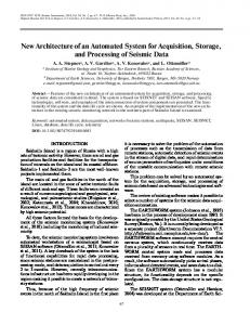
obtaining 3D information using two different image planes, as shown in Fig. 6. The procedure is as follows: 1. The distance from point A1 to point B1 equals the horizontal CCD cell distance from P3 to the centerline of the image multiplied by the real cell size. 2. Angle b1 is calculated using the distance from A1 to B1 and B1 to S1 (lens) in Eq. (1). In the same way, angle b2 is calculated by Eq. (2). 3. Angles c1 and c2 are equal to a1 minus b1 and a2 minus b2, respectively in Eqs. (3) and (4). 4. Angle c3 is equal to 180º minus c1 and c2 as Eq. (5). 5. The horizontal distance from shot 1 to shot 2 in the XY plane is calculated using the coordinates for each in Eq. (6). 6. Given the angles c1 and c2, the horizontal distance from P3 to S1 is calculated by Eq. (7). 7. The coordinates of P3 are calculated by Eqs. (8) and (9). 8. Once the distance between the camera and the object is known, the elevation is also calculated in a similar way, which is described later in this article. The calculation equations are shown as follows (AB means the distance from point A to point B):
3.5 3D Information Extraction With the information of positions and orientations of shots and focal length, 3D information of an object can be extracted by photogrammetric method. This section reviews the procedure for
–1
(1)
b 2 = tan ( A2 B2 ⁄ B2 S2 )
–1
(2)
c1 = a1 – b1
(3)
c2 = a2 – b2
(4)
b 1 = tan ( A1 B1 ⁄ B1 S1 )
o
(5)
c3 = 180 – c1 – c2 2
S 1 S2 = ( X1 – X2 ) + ( Y 1 – Y2 ) S 1 P3 = S1 S2 × sinc2 ⁄ sinc3
2
(6) (7)
Fig. 6. Calculating a Target’s 3D Coordinates − 12 −
KSCE Journal of Civil Engineering
An Automated System for the Creation of an Urban Infrastructure 3D Model using Image Processing Techniques
X3 = X1 + S1 P3 × cosc1
(8)
Y3 = Y1 + S1 P3 × sinc1
(9)
In this algorithm, we assume that the distance from the CCD sensor to the center of the lens equals the focal length. Most consumer class digital cameras, like the cameras used in experiments of this paper use automatic focus, which adjusts the locations of the CCD sensors to produce a clear image. If the object is closer to the camera, the CCD sensor moves away from the lens. In contrast, if the object is far away from the camera (about 10 m), the CCD sensor moves closer to the lens in order to capture a sharp image. A sketch of CCD sensor location is shown in Fig. 7. We assume that the height of the object is 10 m, the distance from the object to the lens is 10 m, and the focal length of the lens is 6.5 mm. The ideal distance from the CCD sensor to the lens is 6.504 mm, which is almost the same as the focal length. The details of the calculations are as follows (AB means the distance from point A to point B): – 1 BB –1 10 × 10 o a = tan ⎛ ---------1⎞ = tan ⎛ -------------------⎞ = 89.963 ⎝ OF ⎠ ⎝ 6.5 ⎠ 3 – 1 ⎛ BB ⎞ –1 10 × 10 o b = tan ⎜ ---------1-⎟ = tan ⎛ -------------------3⎞ = 45 ⎝ ⎠ 10 × 10 ⎝ OB1⎠
(10) (11)
o
6.5 × sin( 180 – a ) OB = ------------------------------------------- = 9.198 mm sinc o
OA1 = OA × cosb = 9.198 × cos45 = 6.504 mm
Fig. 8. Indoor Experiment for 3D Information Extraction: (a) Shot 1, (b) Shot 2, (c) Extracted Result of (a), (d) Extracted Result of (b)
The length of the green line was 62 mm and the pixel distance derived from the image processing results was 41.05. The real pixel size of the CCD array was estimated as follows:
(12)
By Eq. (10), the pixel size of the CCD array 6.5 × 62 –3 = ------------------------------ = 9.82 × 10 mm 1000 × 41.05
(13)
In the proposed application, most of the objects we wish to image are more than 10 m away from the camera. The difference of 0.004 mm can be ignored. In Eq. (1), B1 S1 and B2 S2 are equal to the focal length of the digital camera. An experiment was designed to test the feasibility of the algorithm. A piece of paper marked with a green line and a piece of paper marked with a purple line were posted on a wall. The distance between the left edges of the two lines was 374 mm. The distance between the two shots was 500 mm. The axes of the two shots were perpendicular to the wall, and the distances between the lenses and the wall were both 1000 mm. All images were taken at a focal length of 6.5 mm. The images are shown in Figs. 8(a) and 8(b). The extracted targets are shown in Figs. 8(c) and 8(d). The pixel size of the CCD array is unknown, but the distance between the green line and the lens of the camera was 1000 mm.
In Fig. 8(c), the pixel coordinates of the top-left point on the purple line were (572.5, 239.5), while the pixel coordinates of the same point on the green line were (237.5, 241.5) in Fig. 8(d). We assumed that the widths of the CCD cells of this camera were equal to their lengths. The coordinates of the left edge of the purple line were calculated as (377.0, 987.4). Compared with the actual measurement, which was (374, 1000), the distance error was only 13 mm, resulting in the error rate of 1.3%.
4. Field Experiment for 3D Information Extraction To further evaluate the photogrammetric methodology of obtaining 3D information using two different image planes, a field experiment was performed at an office site consisting of buildings and warehouse structures. Twelve base points and 50 building corners on the site were selected as candidate locations for
Fig. 7. Schematic for the Calculation of the CCD Sensor Location Vol. 16, No. 1 / January 2012
(14)
− 13 −
Junhao Zou, Byungil Kim, Hyoungkwan Kim, and M. Al-Hussein
the field test. The plan of the office site and the locations of the base points and building corners are shown in Fig. 9. The measurements obtained by our camera-based system were compared with those of a total station, which is an electronic and optical surveying instrument, in order to check the accuracy and applicability of the proposed methodology. The images were taken by a 7.1 MP digital camera with a focal length ranging from 6.7 mm to 20.1 mm. The focal length of the camera was fixed at 6.7 mm during this experiment. Although the camera used in this experiment had a 1/2.33” CCD, the actual size of each cell on the CCD array was unknown. An image that covers Base Point 8 to Base Point 11 was used to estimate the size of each CCD cell. The height of the prism and the distances between the base points were 2.6 m and 32.40 m, respectively. The pixel size was calculated to equal 1.928×10⁻³ mm. In this experiment, a few pictures were taken with backlighting. The edges of two overlapping buildings could not be detected in backlit photos, although the two buildings were different colors. The edges of these buildings were manually selected. Out of the 50 building corners, a total of 26 building corners were chosen to be measured by the digital camera for the calculation of northing and easting. Each building corner was measured twice by the camera, and the average was used to calculate the location; the results are shown in Table 1. The average of the errors of the 26 calculated locations is 2.741 m, with a standard deviation of 4.527 m. From Fig. 10, it is easy to find that the errors of the calculated locations increase significantly when either angle c1 or c2 is less than 5o. Fig. 11. shows the distributions of errors of c1 and c2. The average error of c1 and c2 is 0.52o
and the standard deviation is 0.55o. Compared with Fig. 11, the errors of locations varies much greater due to the reviewed photogrammetric method. The location of target point is determined by distance between two shot location, sinc1 and sinc2 based on Eq. (7). If either c1 or c2 is less than 5o, an error of 1o in angle c1 or c2 results in at least a 20% error of the calculated P3 S1 (Fig. 6). In contrast, an error of 1o causes only a 3% error of the same calculation when the angles of c1 and c2 are larger than 30o. Thus, if data obtained when either c1 or c2 is less than 5o are removed from Table 1, the average of the errors of the remaining 20 calculated locations is reduced to 0.908 m and the standard deviation is reduced to 0.718 m. The average length of P3 S1 is 59.288 m, and the average error of the calculated location is then approximately 1.5%. Therefore, conditions in which either c1 or c2 is less than 5o should be avoided. The elevations of the remaining 20 points were calculated as shown in Table 2. The average of the errors is 0.322 mm, with a standard deviation being 0.223 mm. Based on the sizes of the objects that were successfully detected by our system, the accuracies of the captured coordinates and elevation information drawn from 2D images is considered to meet the requirements necessary for a useful 3D model system.
5. Conclusions We presented an image database system for effective management of urban infrastructure. The framework of the proposed system defines how input data, such as image data, shot information (time, location, and elevation), and target features (color, size, and shape) are transformed into a 3D model of a city; the
Fig. 9. Plan of the Office Site and Locations of the Surveyed Points − 14 −
KSCE Journal of Civil Engineering
An Automated System for the Creation of an Urban Infrastructure 3D Model using Image Processing Techniques
Table 1. Calculated Coordinates Compared with Actual Coordinates Point No.
Actual Northing
Actual Easting
Calculated c1 (o)
Actual c1 (o)
Calculated c2 (o)
Actual c2 (o)
Calculated Northing
Calculated Easting
100 101 102 104 105 110 111 112 113 114 115 116 117 119 120 121 122 123 126 127 128 134 135 136 137 148
5936890.121 5936890.115 5936889.995 5936890.967 5936891.175 5936917.087 5936932.966 5936946.897 5936947.165 5936971.796 5936980.04 5936980.08 5936980.335 5936964.464 5936933.105 5936917.167 5936994.552 5936994.682 5937007.185 5937007.061 5937004.804 5936856.773 5936856.958 5936858.984 5936859.055 5936915.683
28598.23 28600.512 28576.184 28609.105 28643.298 28602.634 28602.475 28554.656 28536.564 28554.513 28554.382 28568.861 28608.133 28624.46 28609.859 28610.045 28608.055 28620.506 28620.4 28607.859 28607.796 28609.29 28643.503 28581.671 28596.695 28624.788
22.34 21.14 32.03 18.28 11.61 3.55 13.49 33.80 4.77 170.01 169.74 142.19 13.07 25.27 19.96 11.36 147.79 169.73 88.33 56.95 59.69 6.38 29.94 23.31 15.10 1.44
21.82 21.12 31.98 18.25 12.71 2.29 14.34 31.50 3.97 170.20 169.07 142.35 12.39 26.07 18.75 11.36 147.79 169.73 88.33 56.95 59.56 7.44 30.39 23.7 15.44 0.59
48.64 50.81 28.01 64.25 135.00 7.06 24.25 15.84 2.96 4.65 3.35 6.44 76.51 114.43 32.53 80.27 12.32 4.10 12.34 13.67 15.51 38.8 14.41 16.09 60.00 169.72
48.07 51.23 28.80 65.14 134.28 8.71 25.94 15.99 1.65 3.07 3.58 6.69 75.30 114.44 32.53 80.08 12.66 3.79 12.16 14 15.51 38.8 14.28 16.16 59.94 169.89
5936889.517 5936890.236 5936890.55 5936891.087 5936893.457 5936917.742 5936933.766 5936946.155 5936957.344 5936971.214 5936979.75 5936979.732 5936981.487 5936964.814 5936933.923 5936917.136 5936993.304 5936998.793 5937006.752 5937007.488 5937004.786 5936856.036 5936857.012 5936858.915 5936858.896 5936917.241
28598.142 28600.129 28575.187 28608.568 28642.400 28592.142 28601.643 28552.638 28533.320 28534.811 28554.383 28569.232 28607.645 28622.292 28609.421 28610.033 28608.715 28620.078 28620.390 28608.140 28607.856 28608.167 28643.145 28582.140 28596.771 28631.439
Errors of Calculated Locations 0.611 0.401 1.141 0.550 2.453 10.513 1.154 2.150 10.684 19.711 0.290 0.509 1.251 2.196 0.928 0.034 1.411 4.133 0.433 0.512 0.062 1.344 0.362 0.474 0.176 6.831
Table 2. Calculated Elevations Compared with Actual Elevations Point No. 100 101 102 104 105 111 112 116 117 119 120 121 122 126 127 128 134 135 136 137
Calculated Distance from Camera 32.652 31.345 50.659 26.118 31.082 38.339 73.440 56.232 22.756 46.553 21.800 9.983 31.765 20.444 23.556 26.002 53.789 43.501 14.346 28.714
Vol. 16, No. 1 / January 2012
Vertical Distance to the Center of Image 415.5 656.5 283.5 582.5 407.5 63.5 328.5 208.5 703.5 267.5 203.5 477.5 215.5 475.5 387.5 554.5 328.5 358.5 1001.5 482.5
Calculated Elevation above Camera 3.904 5.921 4.133 4.378 3.645 0.701 6.942 3.374 4.607 3.583 1.277 1.372 1.970 2.797 2.627 4.149 5.085 4.488 4.134 3.987 − 15 −
Elevation of Camera 675.159 675.159 675.159 675.159 675.159 675.249 675.249 675.249 675.249 675.263 675.159 675.159 675.249 674.822 674.822 674.822 674.527 674.527 675.272 675.272
Calculated Elevation 679.063 681.080 679.292 679.537 678.804 675.950 682.191 678.623 679.856 678.846 676.436 676.531 677.219 677.619 677.449 678.971 679.612 679.015 679.406 679.259
Actual Elevation 679.326 680.878 679.326 679.339 679.339 676.298 681.651 679.465 679.437 679.073 676.444 676.444 677.866 677.997 677.997 679.38 679.339 679.339 679.362 679.362
Error in Elevation 0.263 0.202 0.034 0.198 0.535 0.348 0.540 0.842 0.419 0.227 0.008 0.087 0.647 0.378 0.548 0.409 0.273 0.324 0.044 0.103
Junhao Zou, Byungil Kim, Hyoungkwan Kim, and M. Al-Hussein
Acknowledgements This work was supported by a grant (2010-0014365) from the National Research Foundation and Ministry of Education, Science and Technology of Korea. The writers also would like to express their appreciation to the City of Edmonton, AB, Canada and Siri Feranando, Engineering Manager of Drainage Services, City of Edmonton for allowing the experiment to be conducted at the Coronation Yard.
References Fig. 10. Distributions of Errors in Distance Calculated Using Photogrammetric Method
Fig. 11. Distributions of Absolute Value of Errors of c1 and c2 Calculated using Photogrammetric Method
system architecture defines the core system components, such as user interface, image data acquisition equipment, image processing module, 3D information extraction module, and 3D model generation module. We focused on the design of the photogrammetry based 3D information extraction module, which is an automated image processing system. Laboratory and field experimental results showed that our automated system has the potential to efficiently develop large-scale 3D models of the streets of a municipality. Image quality was an important factor determining the accuracy of 3D information. Image processing does not generate useful information if the original images do not include useful information. If the edges of the buildings seen in images are not clear, they cannot be accurately detected. In future studies, a more advanced digital camera with higher resolution will be applied, and the camera will be mounted on a vehicle equipped with a GPS and a gyroscope. The vehicle’s schedule and route will be planned carefully to increase the level of automation by eliminating complicating factors such as backlighting. The methodology of 3D information extraction will also be applied to the measurement of structural damage in a range of urban infrastructures. Such proactive infrastructure monitoring will ensure timely management decisions that lead to safe and efficient infrastructure operations.
Fruh, C. and Zakhor, A. (2003). “Constructing 3D city models by merging aerial and ground views.” IEEE Computer Graphics and Applications, Vol. 23, No. 6, pp. 52-61. Gotoh, T., Kudo, M., Toyama, J., and Shimbo, M. (1999). “Geometry reconstruction of urban scenes by tracking vertical edges.” Proceedings of the Third International Conference on KnowledgeBased Intelligent Information Engineering Systems, Adelaide, Australia. Hyyppa, J., Jaakkola, A., Hyyppa, H., Kaartinan, H., Kukko, A., Holopainen, M., Zhu, L., Vastaranta, M., Kaasalainen, S., Krooks, A., Litkey, P., Lyytikainen-Saarenmaa, P., Matikainen, L., Ronnholm, P., Chen, R., Chen, Y., Kivilahti, A. and Kosonen, I. (2009). “Map updating and change detection using vehicle-based laser scanning.” Proceedings of Urban Remote Sensing Joint Event, Shanghai, China. Konkol, J. and Prokopski, G. (2007). “The necessary number of profile lines for the analysis of concrete fracture surfaces.” Structural Engineering and Mechanics, Vol. 25, No. 5, pp. 565-576. Lafarge, F., Descombes, X., Zerubia, J., and Deseilligny, M. (2006). “An automatic 3D city model: A Bayesian approach using satellite images.” Proceedings of IEEE International Conference on Acoustics, Speech and Signal Processing, Toulouse, France. Linder, W. (2006). Digital photogrammetry: A practical course, Springer. Peng, J., Najjar, M., Cappelle, C., Pomorski D., Charpillet, F., and Deeb, A. (2009). “A novel geo-localisation method using GPS, 3D-GIS and laser scanner for intelligent vehicle navigation in urban areas.” Proceedings of International Conference on Advanced Robotics, Munich, Germany. Poullis, C. and You, S. (2009), “Automatic reconstruction of cities from remote sensor data.” Proceedings of IEEE Computer Society Conference on Computer Vision and Pattern Recognition, Miami Beach, Florida, USA. Regez, B., Zhang, Y., Chu, T., Don, J. and Mahajan, A. (2008). “Inplane bulk material displacement and deformation measurements using digital image correlation of ultrasonic C-scan images.” Structural Engineering and Mechanics, Vol. 29, No. 1, pp. 113-116. Rottensteiner, F., Trinder, J., and Clode, S. (2005). “Data acquisition for 3D city models from LIDAR: Extracting buildings and roads.” Proceedings of IEEE International Geoscience and Remote Sensing Symposium, Seoul, Korea. Styliadis, A. D. (2007). “Digital documentation of historical buildings with 3-d modeling functionality.” Automation in Construction, Vol. 16, No. 4, pp. 498-510. Tarsha-Kurdi, F., Landes, T., and Grussenmeyer P. (2007). “Joint combination of point cloud and DSM for 3D building reconstruction using airborne laser scanner data.” Proceedings of IEEE Urban Remote Sensing Joint Event, Paris, France.
− 16 −
KSCE Journal of Civil Engineering
An Automated System for the Creation of an Urban Infrastructure 3D Model using Image Processing Techniques
Tolt, G. and Ahlberg, S. (2007), “3D urban models from laser radar data.” Proceedings of IEEE Urban Remote Sensing Joint Event, Paris, France. Tsai, F., Teo, T., Chen, L., and Chen, S. (2009), “Construction and visualization of photo-realistic three-dimensional digital city.” Proceedings of Urban Remote Sensing Joint Event, Shanghai, China. Verma, V., Kumar, R., and Hsu, S. (2006). “3D building detection and modeling from aerial LIDAR data.” Proceedings of IEEE Computer Society Conference on Computer Vision and Pattern Recognition , New York, USA. Wang, M., Bai, H., and Hu, F. (2008). “Automatic texture acquisition for 3D model using oblique aerial images.” Proceedings of IEEE International Conference on Intelligent Networks and Intelligent Systems, Wuhan, China. Wikipedia (2010). Google street view, (Jul. 15, 2010). Wu, Y., Kim, H., Kim, C., and Han, S. H. (2010). “Object recognition in
Vol. 16, No. 1 / January 2012
construction site images using 3D CAD-based filtering.” Journal of Computing in Civil Engineering, Vol. 24, No. 1, pp. 56-64. Xiao, Y., Lim, S. K., Tan, T. S., and Tay, S. C. (2004). “Feature extraction using very high resolution satellite imagery.” Proceedings of 2004 IEEE International Geoscience and Remote Sensing Symposium, Anchorage, Alaska. Yilmaz, H. M., Yakar, M., and Yildiz, F. (2008). “Documentation of historical caravansaries by digital close range photogrammetry.” Automation in Construction, Vol. 17, No. 4, pp. 489-498. Zhu, L., Hyyppä, J., Kukko, A., Jaakkola, A., Lehtomäki, M., Kaartinen, H., Chen, R., Pei, L., Chen, Y. Hyyppä, H., Petri, R., and Haggren, H. (2009). “3D city model for mobile phone using MMS data.” Proceedings of Urban Remote Sensing Joint Event, Shanghai, China. Zou, J. and Kim, H. (2007). “Using HSV color space for construction equipment idle time analysis.” Journal of Computing in Civil Engineering, Vol. 21, No. 4, pp. 238-246.
− 17 −