of 23 programs and respectively achieves a performance im- provement of 22% ...... and by the Austrian Research Promotion Agency under con- tract nr. 834307 ...
An Automatic Input-Sensitive Approach for Heterogeneous Task Partitioning Klaus Kofler, Ivan Grasso, Biagio Cosenza and Thomas Fahringer Institute of Computer Science University of Innsbruck, Austria
{klaus,grasso,cosenza,tf}@dps.uibk.ac.at ABSTRACT
1.
Unleashing the full potential of heterogeneous systems, consisting of multi-core CPUs and GPUs, is a challenging task due to the difference in processing capabilities, memory availability, and communication latencies of different computational resources. In this paper we propose a novel approach that automatically optimizes task partitioning for different (input) problem sizes and different heterogeneous architectures. We use the Insieme source-to-source compiler to translate a singledevice OpenCL program into a multi-device OpenCL program. The Insieme Runtime System then performs dynamic task partitioning based on an offline-generated prediction model. In order to derive the prediction model, we use a machine learning approach based on Artificial Neural Networks (ANN) that incorporates static program features as well as dynamic, input sensitive features. Principal component analysis have been used to further improve the task partitioning. Our approach has been evaluated over a suite of 23 programs and respectively achieves a performance improvement of 22% and 25% compared to an execution of the benchmarks on a single CPU and a single GPU which is equal to 87.5% of the optimal performance.
In the past few years, heterogeneous computing systems have emerged as mainstream and cost-effective means for scaling. Compared to traditional homogeneous systems, they offer high peak performance and energy efficiency. Not surprisingly, three of the ten fastest supercomputers in the world are heterogeneous systems [5], consisting of nodes with multi-core CPUs and GPUs. The transition from homogeneous to heterogeneous architectures is challenging with respect to the efficient utilization of the hardware resources and the reuse of the software stack. This problem has drawn great interest from researchers and industry, leading to the proposal of several programming models including HMPP [2], OpenACC [3], CUDA [27] and OpenCL [22]. OpenCL (Open Computing Language) is the first open standard for cross-platform parallel computing, supported by many hardware vendors such as AMD, ARM, IBM, Intel, and NVIDIA. OpenCL supports a wide range of hardware through a lowlevel high performance abstraction layer, supporting the development of programs without knowledge of the underlying architecture. Nevertheless, writing programs for heterogeneous systems remains a challenging task due to the difference in processing capabilities, memory availability, and communication latencies of different computational resources (called devices in OpenCL).
Categories and Subject Descriptors D.3.2 [Language Classifications]: Concurrent, distributed, and parallel languages; D.3.4 [Processors]: Code generation/Compilers; C.1.3 [Other Architecture Styles]: Heterogeneous (hybrid) systems
General Terms Languages, Algorithms, Performance
Keywords heterogeneous computing, compilers, GPU, task partitioning, code analysis, machine learning, runtime system
Permission to make digital or hard copies of all or part of this work for personal or classroom use is granted without fee provided that copies are not made or distributed for profit or commercial advantage and that copies bear this notice and the full citation on the first page. To copy otherwise, to republish, to post on servers or to redistribute to lists, requires prior specific permission and/or a fee. Copyright 20XX ACM X-XXXXX-XX-X/XX/XX ...$15.00.
1.1
INTRODUCTION
Motivation
As heterogeneous computing opens many new opportunities for developing parallel algorithms, our work is motivated by the additional challenges and complexity that it also introduces. One of the challenges is the distribution of tasks (i.e. task partitioning) among the available OpenCL devices in order to maximize the system performance. Task partitioning defines how the total workload (all threads of a program) is distributed among several computational resources. It is important to understand that the best performing task partitioning is likely to change with different applications, different (input) problem sizes, and different hardware configurations. We justify our statement presenting a case study with two programs which are part of our test cases: linear regression and reduction. The programs have been executed with different problem sizes and varying task paritionings. We measured the execution times on two heterogeneous target architectures, consisting of one CPU and two GPUs (the target architecture configurations are detailed in Table 3). The results of these experiments are shown in Figure 1.
one CPU
best hybrid one GPU two GPUs
execution time (sec)
execution time (sec)
6.4E+01 3.2E+01 1.6E+01 8.0E+00 4.0E+00 2.0E+00 1.0E+00 5.0E-01 2.5E-01 1.3E-01 6.3E-02 3.1E-02 1.6E-02 7.8E-03 3.9E-03 2.0E-03
6.4E+01 3.2E+01 1.6E+01 8.0E+00 4.0E+00 2.0E+00 1.0E+00 5.0E-01 2.5E-01 1.3E-01 6.3E-02 3.1E-02 1.6E-02 7.8E-03 3.9E-03 2.0E-03 9.8E-04 4.9E-04
nr. of threads
best hybrid one GPU two GPUs
nr. of threads
(a) Linear regression on mc1
(b) Linear regression on mc2
5.0E-01
2.5E-01
2.5E-01
1.3E-01
1.3E-01
6.3E-02
6.3E-02 3.1E-02 1.6E-02
one CPU
7.8E-03
best hybrid
3.9E-03
one GPU
2.0E-03
two GPUs
execution time (sec)
execution time (sec)
one CPU
3.1E-02 1.6E-02 7.8E-03
one CPU
3.9E-03
best hybrid
2.0E-03
one GPU
9.8E-04
two GPUs
9.8E-04
4.9E-04
4.9E-04
2.4E-04
nr. of threads
(c) Reduction on mc1
nr. of threads
(d) Reduction on mc2
Figure 1: Performance behavior of two programs on different target architectures with varying problem size (i.e. the number of threads). Each chart shows execution times (in seconds) in logarithmic scale (y-axis) with different number of threads (work items in OpenCL) (x-axis). Detailed hardware descriptions of the target architectures mc1 and mc2 are shown in Table 3. On the first target architecture (mc1, see Table 3) for small problem sizes, the GPU is less effective and the one CPU task partitioning delivers the best performance for both applications. However, for specific problem sizes, a hybrid task partitioning (using the CPU as well as one or two GPUs) or a GPU only task partitioning is preferable. On the second target architecture (mc2, see Table 3), linear regression performs best on one GPU for smaller problem sizes while reduction reaches the best performance with one CPU. For increasing problem sizes the GPUs become more effective and linear regression should be distributed over two GPUs for both mc1 and mc2. The reduction program exhibits a different behavior for larger problem sizes, favoring hybrid solutions which outperform any homogeneous configuration by up to 44% and 19% on mc1 and mc2, respectively. These experiments demonstrate that even for a single application, the optimal partitioning considerably depends on the problem size and the capabilities of the hardware. Another important aspect of heterogeneous computing is the difficulty of writing multi-device programs (i.e. a single program which can be executed on multiple devices concurrently). Since current state-of-the-art compilers are not capable of automatizing this complex task, new tools are needed in order to facilitate the conversion of existing programs to heterogeneous systems.
In this paper we present an automatic, problem size sensitive compiler-runtime method for task partitioning of OpenCL programs on heterogeneous systems. Our work is based on machine learning which effectively combines compile time analysis with runtime feature evaluation to predict the optimal task partitioning for every combination of program, problem size and hardware configuration. The contributions of this paper are as follows: • We propose and implement a novel compiler-runtime framework for auto-generation of multi-device OpenCL code and optimized task partitioning on heterogeneous systems. Our framework is portable to any OpenCL environment with an arbitrary number of devices. Our task partitioning approach is based on an offline generated problem size sensitive model, which is capable of outperforming the CPU/GPU only strategy by 22% and 25%, respectively. Our experimental results demonstrate the capabilities of our approach using 23 different applications on two different heterogeneous multi-device systems. • We show that Principal Component Analysis (PCA) does improve the performance of dynamic task partitioning system by 2% to 7%, depending on the used machine learning technique and target architecture.
compile time 1
Input Codes
Analyzer
runtime
Backend 3
2
compile time 1
Multi-device Runtime Code
Input Code
Analyzer
5
training phase
7
Model
Execution
4
Multi-device Runtime Code
5
Runtime Features
Model
Runtime System
Trainer
Backend
Code Features
Runtime Features
6
runtime
4 2
Code Features
3
Measurements
Runtime System 7 Execution
6 Configuration
Parallel Heterogeneous Platform
Parallel Heterogeneous Platform
(a) Training phase
(b) Deployment phase Figure 2: Framework Overview
• We present an analysis of different machine learning techniques suitable to solve the automatic task partitioning problem and show that Artificial Neural Networks (ANN) outperform Support Vector Machines (SVM) for the presented use case. • We empirically demonstrate the benefits of our machine learning based approaches compared to traditional static task partitioning techniques. The remainder of this paper is organized as follows. The next section gives an architectural overview of the Insieme Compiler and Runtime framework. Section 3 describes the partitioning problem and the generation of the machine learning models. Section 4 presents the experimental methodology. Section 5 discusses the experimental results. Section 6 presents related works and Section 7 concludes the paper.
2.
FRAMEWORK OVERVIEW
Heterogeneous systems are difficult to program, and moreover the performance capability of individual devices can vary significantly across different applications and problem sizes which often makes static, problem size insensitive distribution techniques unsuitable. The Insieme Compiler and Runtime framework [1] relieves the developer from this difficult task. It consists of a source-to-source compiler and a runtime system. The Insieme Compiler translates singledevice OpenCL programs (i.e. OpenCL programs which use only one computational resource) into multi-device OpenCL programs. The Insieme Runtime System distributes the computation among the available devices to effectively exploit the performance capabilities of a heterogeneous system.
2.1
Architecture
Figure 2 illustrates the architecture of the proposed framework, highlighting two main phases: training and deployment. The labels (1-7) in Figure 2(a) and Figure 2(b) explain the processing of a program within the Insieme framework. The goal of the training phase is to build a task partitioning prediction model. Any previously unseen target architecture can be supported by generating a new model for it. Since the model generation is done automatically, our approach can be ported to any heterogeneous system without user intervention. To build a model, a set of OpenCL programs are provided to the system and translated into the Insieme parallel intermediate representation (INSPIRE, see
Section 2.2) by the code analyzer (1). From this representation, the features of the program (static program features) are extracted and stored in a database (2). The intermediate representation of the program is then passed to the backend which generates multi-device OpenCL code (3). Once generated, the new program will be executed with various problem sizes and the available task partitionings. The obtained performance measurements (4), together with the problem size dependent features of the program (i.e. runtime features), are collected and added to the database (5). After these steps have been accomplished for all programs, the trainer uses the features and the performance measurements stored in the database (6) to generate a task partitioning prediction model (7). In the deployment phase a new OpenCL program is provided to the analyzer (1) for optimizations, the static features are extracted (2) and the intermediate representation is passed to the backend (3) which generates a multi-device OpenCL program (4). When the program is executed, the runtime features are provided to the previously trained model (5), which combines them with the static program features to predict the best task partitioning for the current program with the selected problem size (6). Finally, the runtime system executes the program on the given hardware using the predicted task partitioning (7).
2.2
Implementation
We have implemented a powerful framework for code transformations and program analysis for heterogeneous parallel systems as part of Insieme [1]. It consists primarily of two components: a source-to-source compiler and a runtime system. The compiler translates OpenCL input code to an Intermediate Representation (IR) and back to OpenCL. This IR offers a formal and compact representation of programs that facilitates code analysis and transformation. The Insieme Runtime System is responsible for the execution and scheduling of the generated programs. It is capable of partitioning and distributing tasks over heterogeneous computing devices using interchangeable scheduling policies. The input for the Insieme Compiler abc is a single-device OpenCL program. An OpenCL program consists of a host and a device part. The host part runs on the CPU and is responsible for setting up the OpenCL devices (e.g. a GPU or the CPU itself). The device part (called kernel ) is a data-parallel task and describes the computations performed by a single thread (called work item in OpenCL). During the program execution, a certain number of work items is
generated and executed in parallel. The number of work items generated increases with the input problem size. The exchange of data between the host and the compute devices is implemented through memory buffers, that are passed as separate arguments to the kernel. The translation of the OpenCL input code into IR code occurs in two distinct steps. In the first step, the Insieme Compiler uses the open source Clang C frontend [7] to generate an Abstract Syntax Tree (AST) from the input code. In a second step, the AST is transformed to the Insieme parallel intermediate representation (INSPIRE [1]) on which analyses and transformations are performed. In order to distribute a task, the Insieme Compiler analyzes the generated IR of the input program. It collects the subscripts of all buffer accesses in order to derive the buffer’s access pattern. This analysis identifies whether a buffer should be replicated or distributed evenly among several devices. After collecting all the access patterns, the analysis checks if the access expression is (a) a constant, (b) the result of a convex function depending on the thread id, or (c) something else. If only accesses of type (b) occur, the buffer is split among all devices (i.e. buffer is splittable). If accesses of type (a) or (c) happen, part of it (a) or the entire buffer (c) has to be copied to every device (i.e. the buffer is non-splittable). In case of (a) and (c), the amount of data to be transferred increases linearly with the number of devices used. Obviously, copying the same data to each device is only feasible if there are only read accesses to these buffers. When write accesses of type (a) or (c) occur, our framework is not capable of distributing the kernel. A kernel can be distributed over several devices if and only if all its buffers with write accesses are splittable. However, due to the limited synchronization capabilities of OpenCL, in most kernels use access pattern (b) for their write accesses, which means they are splittable. The access pattern analysis is based entirely on the device code. However, also the host code has to be adapted according to the results of the access pattern analysis in order to guarantee the correct distribution of data. For this reason, the Insieme Compiler connects host and device code during the translation of the Clang AST into IR, enabling the analysis of the entire program. After the analysis, the IR is translated by the backend to a multi-device OpenCL program. The generated code is semantically equivalent to the input code, but its kernels can be distributed among a generic number of devices by the Insieme Runtime System. This implies that some buffers are replicated while others are distributed over the selected devices, depending on their access pattern inside the kernel. To select the task partitioning a priori, the runtime system employs a model generated by machine learning. This model is based on static program features extracted at compile time and problem size sensitive features collected at runtime. A detailed description of how we extract features and build this model can be found in Section 3.
2.3
Limitations
While the Insieme framework can be used to optimize the performance of many programs on heterogeneous systems, it also has limitations that leave room for future improvement. At the current stage, the buffer analysis and task partitioning are executed individually on each kernel. In programs with multiple kernels, this can cause unnecessary data trans-
fers since the output of each of them must be copied back to the host in order to be redistributed with a new task partitioning. Device-specific optimizations are not in the scope of this publication, although our machine learning guided task partitioning could potentially support it. We are aware of the opportunities that this approach can offer and we will investigate it in future work. Other restrictions are related to scattered data accesses and atomic operations, both performed on buffers in global memory. For scattered accesses on buffers, the analysis distinguishes two cases: read-only and read-write buffers. In the first case, the entire buffer will be copied to each device including data that is not needed. In the second case the kernel will be not distributed, since the gathering and merging of writes from different devices is not yet supported. Regarding the use of atomic operations on buffers, OpenCL does not provide any means to implement such operations over multiple devices, therefore Insieme currently does not support kernels with atomic operations. Our approach cannot deal with irregular workloads due to the difficulty to statically predict an optimized task partitioning for such cases.
3.
PARTITIONING PARALLEL TASKS
Data-parallel tasks can often be split into smaller subtasks and distributed across multiple devices. However, finding an efficient partitioning is not trivial. As will be explained in Section 5 and also pointed out by other studies [18], a dynamic scheduling approach may not lead to an optimal solution, mostly due to the large difference in performance and transfer bandwidth of the individual devices. Therefore our approach, based on analysis of the program structure and input data, tries to predict the optimal partitioning for an OpenCL program a priori. This section describes the extraction of features and the construction of the machine learning model, used to predict a partitioning.
3.1
Predicting the Optimal Partitioning
Our overall approach requires to build a model using machine learning in order to predict a task partitioning p from a vector of features that describes the essential characteristics of a program as well as the current problem size. Each task partitioning is characterized by a tuple of n integer values for a target architecture with n devices. Each value represents the percentage of work that is executed on a particular device. The set P contains all possible partitionings over the available devices with a granularity of 10% and the predicted task partitioning p should be as near as possible to the best task partitioning in terms of performance. As done in [18] we choose a granularity of 10% since this is a good compromise between granularity and number of task partitionings.
3.2
Extracting Features
The feature extraction consists of two phases. In the first phase, all the features that can be statically inferred from the intermediate representation are extracted. This is done during the source-to-source compilation step of the Insieme Compiler. In the second phase, the Insieme Runtime System determines the values of all problem size dependent runtime features. This phase takes place when a program is executed, since the problem size is unknown at compile time.
(a) Features selected by Greedy Feature Selection for mc1 Rk. static program features 2 OpenCL built-in functions 3 Number of branches / number of statements 4 Scalar float operations /number of statements Rk. Runtime features 1 Data transfer size for splittable buffer (device to host) 5 Number of global work items 6 Data transfer size for splittable buffer (host to device) 7 Runtime feature Nr. 3 / total number of arith. operations
MSE 76.3 64.4 61.1 MSE 99.7 60.0 47.6 47.5
(b) Features selected for mc2 Rk. static program features 1 Number of branches / number of statements 2 Scalar float operations / number of statements 4 OpenCL built-in functions / number of statements 6 Scalar int operations / number of statements 7 Vector float operations / number of statements 8 Number of loops / number of statements 9 Scalar int operations 10 Vector float operations Rk. Runtime features 3 Data transfer size for splittable buffer (host to device) 5 Data transfer size for splittable buffer (device to host)
MSE 91.6 75.8 66.9 56.5 52.2 48.6 47.5 46.9 MSE 69.6 64.0
Table 1: Static program and runtime features used by our approach determined using the Greedy Feature Selection [30] ranked with their selection order along with the mean squared error (MSE) on the training dataset using an SVM. The feature extractor needs to know the execution count of each feature relevant statement. If it is not possible to derive the execution count at compile time (for instance, if loop bounds depend on input data), the feature extractor assumes a loop iteration count of 100. This means that every static feature that appears in a loop is multiplied by 100. If loops are nested, this rule is applied recursively. The resulting value may not be realistic in many cases. However, our goal is not to estimate the absolute execution times but instead compare relative execution times for different devices. Therefore, it is sufficient to consider whether feature relevant statements occur outside, inside or within nested loops. The compiler is also responsible for the generation of one univariant linear polynomial for each runtime feature, which takes the problem size as input. The generated polynoms are evaluated during the second phase of the feature extraction to calculate the actual values of the runtime features. The features we used to train our framework are subdivided in static program features (extracted from the intermediate representation during the source-to-source translation process) and runtime features (calculated by the runtime system when the program is executed). Most static program features count the occurrence of certain activities, like arithmetic operations, memory accesses, or OpenCL built-in functions (e.g. log or cos). Others describe the ratio between two characteristics (e.g. the ratio between computation and memory accesses or the ratio between number of branches and all instructions). All runtime features depend on the problem size. Apart from the problem size itself, they describe how much data has to be transferred between the host and the devices. We differ between device-to-host and host-to-device transfers and between transfer size for splittable and non splittable buffers. Since splittable buffers are distributed over all devices, the total amount of data to be copied is independent from the number of devices used. In contrast, the transfer size of non splittable buffers scales with the number of devices, since each device must hold a copy of the entire buffer in its memory. We used the Greedy Feature Selection described in [30] and illustrated by Algorithm 1 to select the most important features out of a set of 24 static code features and 9 dynamic runtime features. To select the most important features, a separate model is trained for each single feature s ∈ S. The one of the model which yields the lowest error mse is added
Algorithm 1 Greedy Feature Selection. The features to be used are collected in the set F . 1: S ← non empty set of all features 2: F ← ∅; mse ← ∞; improved ← true 3: while improved do 4: improved ← f alse 5: for all s ∈ S do 6: model ← trainM odel({s} ∪ F ) 7: msetmp ← evaluate(model) 8: if msetmp < mse then 9: mse ← msetmp 10: f ←s . feature selected to be used 11: improved ← true 12: end if 13: end for 14: if improved then 15: S ← S \ {f } 16: F ← F ∪ {f } 17: end if 18: end while
to the set of selected features F . In the next step, a separate model for each remaining feature s and the already selected ones in set F is trained. Again, the feature which gives the lowest error is added to the set of selected features F . We repeat this step until adding another feature will not further improve the error. We performed this greedy algorithm on both target architectures using an SVM. For the feature selection, static code features and dynamic runtime features were treated equally. Table 1 lists the features that we used to train models for our two target architectures. The column Rk. indicates the order in which the features where added. The column MSE shows the means squared error of the model using the current feature and the ones with a lower Rk. The selected features clearly show that on mc1 the dynamic runtime features have a bigger influence on the result, while on mc2 the static features are more important. This underlines the necessity to select the features individually for different target architectures. As shown in Section 5, the combination of the selected static program features and runtime features apparently carry enough information to characterize the behavior of our tested programs.
3.3
Generating Training Data
Training codes description Application Data Transfer to/from Device Vector Addition Matrix Multiplication Black-Scholes Option Pricing Vertex positions in Sine Wave Pattern 2D 3x3 Convolution Molecular Dynamics Simulation Sparse Matrix Vector Multiplication Linear Regression K-Means clustering K-Nearest-Neighbor Classification Symmetric Rank-2k Operations Sobel Filter Median Filter Ray-triangle Intersection Finite-time Lyapunow Exponent Field Calculation Flow Map Calculation Chunked Reduction Perlin Noise Generator Chunked Calculation of the Geometric Mean Mersenne Twister Random Number Generator Bytewise Integer Compression Simulation of a Swinging Pendulum 1
Performance1 on mc1 CPU GPU SVM ANN 90 37 92 98 77 40 93 94 64 49 78 87 82 41 91 93 15 70 34 47 70 50 94 98 81 57 94 99 96 59 97 100 51 59 51 60 86 48 97 98 22 68 45 48 95 24 87 78 75 58 91 97 82 54 96 98 90 62 94 97 77 56 95 94 91 35 60 92 72 41 84 89 94 17 81 73 68 45 81 92 79 41 91 89 77 39 90 94 20 75 20 20
Performance1 on mc2 CPU GPU SVM ANN 84 72 88 94 71 69 87 85 45 79 98 90 65 76 93 95 7 70 83 95 38 82 95 96 68 87 83 94 82 93 98 96 22 74 70 83 76 80 85 88 5 68 69 87 94 49 51 54 51 90 85 85 56 93 90 96 74 98 89 94 59 82 85 84 75 81 81 88 61 73 88 87 83 49 84 85 54 81 94 93 67 72 90 91 70 69 89 95 19 70 58 76
Achieved performance compared to the maximum performance as percentage values as described in Section 5.
Table 2: Description of test cases used for model training and performance of various task partitioning strategies. To train and validate our model we use the set of codes listed in Table 2. As shown in Figure 2(a), all training codes are compiled with the Insieme source-to-source compiler and their static program features are collected in a database. After the compilation, the programs are executed with various problem sizes (9 to 18 problem sizes, depending on the program) and task partitionings, adding to the database information about runtime features and execution times. The set of explored task partitionings depends, as described in Section 3.1, on the number of available devices in the system. In order to generate the training patterns needed for the model generation, we perform an exhaustive search on that set, finding the task partitioning with the best execution time. The size of the search space is defined by the number of experiments multiplied with the number of possible task partitionings. For the number of training codes and the target architectures considered in our study, the search space consists of 355 × 21 = 7455 elements, where 355 corresponds to all problem size/program combinations and 21 is the number of task partitionings. For each combination of test case and problem size we generate one training pattern that combines static and dynamic program features with the best performing task partitioning. Such task partitioning will then be used as target value during the training of our model.
3.4
Building the Model
Based on the training patterns we build a model with one input for each feature (listed in Table 1) and one output, which represents the task partitioning predicted by the model. In our framework the user can choose between Support Vector Machines [12] and Artificial Neural Networks [12] (ANN). As shown in Table 4, SVMs have a much lower training time, while ANNs introduce a lower overhead during the deployment phase and show a higher performance.
During the construction of the model we also evaluate the effect of Principal Component Analysis [12] (PCA) on the result. PCA can be described as the linear projection that minimizes the average projection cost, defined as the mean squared distance between the data points and their projections [29]. In our case this means that a certain number of features is reduced to a smaller number of new features in a lossy way, conserving as much of the original features’ variance as possible. PCA can help to increase the estimation accuracy of models. However, calculating the PCA, which includes the calculation of the features’ eigenvalues and eigenvectors, introduces a notable overhead. This means that applying PCA to all our features, which include some values only available at runtime, would substantially increase the execution time. In order to eliminate this additional overhead, we apply PCA only to the static program features, leaving the runtime features unchanged. In this way we move the overhead of calculating the principal components from runtime to the source-to-source compilation phase. The effect of PCA on our models’ performance is described in Section 5.2.
4.
EXPERIMENTAL METHODOLOGY
This section describes the test cases and the target architectures used in our experiments as well as the evaluation methodology.
4.1
Test Cases
To evaluate the performance of our approach we used a selection of 23 programs (see Table 2). These programs have been drawn from OpenCL vendors example codes, applications from our department and VRC at the Universit¨ at Stuttgart [28], and benchmark suites [13, 16, 10]. After translating the OpenCL input program with the Insieme Compiler, the Gnu Gcc Compiler version 4.6.3 was used to convert the resulting code to binary.
Machine Name mc1 mc2 CPU manufacturer AMD Intel CPUs 2x Opteron 6168 2x Xeon X5650 #CPU cores (HT) 24 12 (24) CPU frequency 1.9 GHz 2.67 GHz #Parallel Ops (SP) 96 48 Peak Performance 364 GFLOPS 256 GFLOPS Memory 32 GB 24 GB Memory Bandwidth 83 GB/s 62 GB/s Compiler GCC 4.6.3 w/ ”-O3” Operating System CentOs 5.8 OpenCL version AMD APP SDK 2.7 GPU manufacturer Ati NVIDIA GPUs Radeon HD5870 GeForce GTX480 #GPU cores 20 15 Core frequency 850 MHz 1401 MHz #Parallel Ops (SP) 1600 480 Peak Performance 2.7 TFLOPS 1.3 TFLOPS Memory 2 GB 1.5 GB Memory Bandwidth 153 GB/s 177 GB/s Connection PCIe 2.0 x16 PCIe 2.0 x16 OpenCL version AMD APP SDK 2.7 CUDA 4.1.1
Table 3: Experimental target architectures. In order to examine the impact of problem sizes on task partitioning we executed each benchmark with varying problem sizes on two target architectures. For each test case we examined 9 to 18 different problem sizes (depending on the amount of memory needed by the program), resulting in 355 training patterns. Each training pattern consists of the static features of a program, its runtime features for a certain problem size as well as the best task partitioning for the given program with the current problem size. To ensure a fair comparison between different task partitionings, we measured the execution time of the kernels including the memory transfer overhead [17]. For each task partitioning, we executed a series of five experiments, recording the average execution time. The result has been validated with the Student’s t test [4], ensuring reliable results with a confidence level of 95%.
4.2
Experimental Setup
The experiments were performed on two different heterogeneous target architectures composed of three OpenCL devices: two GPUs and two multi-core CPUs in a dual-socket infrastructure. While both GPUs represent a separate device, the two CPUs are reported as a single OpenCL device. The first platform, mc1, consists of two AMD Opteron CPUs and two Ati Radeon GPUs, while the second, mc2, holds two Intel Xeon CPUs and two NVIDIA GeForce GPUs. Table 3 gives a more detailed listing of the two systems’ characteristics. As already mentioned in Section 3.1 we use a set of task partitionings. For the target architectures used in this study, consisting of one CPU device and two GPU devices, we characterize each task partitioning with a tuple of three numbers representing the percentage of the workload executed on a specific device. The first number represents the portion to be executed on the CPU while the second and third number represent the percentage for the first and second GPU, respectively. Task partitioning (100, 0, 0), for example, means that the entire workload is assigned to the CPU, while (0, 50, 50) means that the work is distributed evenly among the two GPUs while nothing is assigned to the CPU.
The entire set of task partitionings P is constructed as follows: X ={0, 10, 20, ..., 100} [ � P = (x, 100 − x, 0), (x,
100−x 100−x , 2 ) 2
x∈X
Where X is the set of different percentage values of the workload considered to be executed by the CPU. The remaining workload is then executed by the first GPU or it is distributed evenly among the two GPUs. The resulting set P consists of 21 different task partitionings. From this set P our runtime system tries to select the optimal task partitioning using the prediction model as described in Section 3. To evaluate the performance of our approach we compare the execution times of a program with two different task partitionings. The first task partitioning is proposed by the Insieme Runtime System and the second one is found by an exhaustive search over all task partitionings over the set P . In order to evaluate the quality of our models we do a leave-one-out cross validation [14] on all our training programs of the set C listed in Table 2. To evaluate the model’s performance for a particular program c ∈ C, we train the model with all programs except c. Obviously, this means not leaving out only one training pattern, but all training patterns related to program c (all different problem sizes).
5.
EXPERIMENTAL RESULT
In this Section we report the performance result of our approach. As performance metric we use the achieved percentage of the maximum performance, which can be reached by applying the best task partitioning. We calculate it as follows s = tbest /tactual ∗ 100 where s is the achieved performance in percentage, tbest is the execution time of the best task partitioning (identified with an exhaustive search over all task partitionings used) and tactual is the actual execution time of the selected task partitioning. To combine the performance for several experiments in one value (e.g. the performance for a specific test case using different problem sizes), we simply calculate the average of the performance across these experiments.
5.1
Performance Results
Depending on the target architecture, the problem size and the program, it can be important to select a certain task partitioning, whereas in other cases, several different task partitionings may deliver similar good performance. For instance, as can be seen in Figures 3(a) and 3(b), when executing matrix multiplication with large problem sizes it is very important to distribute the workload over both GPUs. Furthermore, for hybrid solutions it is not important if one or two GPUs are used, since the CPU is always the limiting factor. For smaller problem sizes, in particular for mc2, several task partitionings yield good performance. In contrast to that, on mc1 small matrices should be multiplied on the CPU alone. The penalty for selecting a non-optimal task partitioning for intermediate problem sizes on mc1 is less severe than on mc2.
100%
100%
80%
80%
60%
60%
32768
32768
524288
40%
524288
40%
8388608
8388608
20%
20%
0%
0%
(a) Matrix Multiplication on mc1
(b) Matrix Multiplication on mc2
100%
100%
80%
80%
60%
60%
16384
131072
40%
16384 131072
40%
4194304
4194304 20%
20%
0%
0%
(c) Bytewise Integer Compression on mc1
(d) Bytewise Integer Compression on mc2
Figure 3: Performance behavior of different programs on two target architectures with different problem sizes (e.g. 32768 work items). On the x-axis the various task partitionings are listed while the y-axis shows the achieved performance in %, relative to the best task partitioning (see Section 5). The situation is different when running our integer compression implementation. Figure 3(c) shows that on mc1 with a problem size of 16384 work items, the CPU substantially outperforms all other task partitionings, while on mc2 the difference is much smaller and all task partitionings deliver 40% or more of the maximum performance, as revealed in Figure 3(d). For the larger problem sizes, on both target architectures a hybrid task partitioning delivers the best performance. However, the best performing task partitioning is different for each problem size and target architecture. In this test case, using a heterogeneous distribution can reduce the execution time by up to 23% over any homogeneous task partitioning (including the dual GPU task partitioning). As shown in Figure 1, there are cases in which a single GPU performs better than two GPUs. This behavior can be observed for some data transfer dominated scenarios and is mainly related to the shared connection of the GPUs to the CPU’s main memory. From the 355 training patterns considered for this study, more than 25% deliver best performance when using a hybrid task partitioning.
5.2
Comparison of Different Techniques
For the Insieme Runtime System we tested a variety of models, generated either with a Support Vector Machine [12] (SVM) or an Artificial Neural Network [12] (ANN). For both techniques we used the implementation provided by the Shark library [20]. In this section, we compare the performance of our model-guided runtime system with the performance of the two default strategies which use either one CPU or one GPU. These are the only available options when using the unchanged input programs, without the generation of multi-device code by the Insieme Compiler. Furthermore, without using the Insieme framework, the
Task ParExecution Time titioning Training (sec) Deployment (ms) Performance1 Approach mc1 mc2 mc1 mc2 mc1 mc2 Avg. CPU only 73 58 65.5 GPU only 48 77 62.5 Random 0.12 0.09 44 55 59.5 SVM2 8 8 0.31 0.23 80 78 79.0 ANN2 248 421 0.07 0.07 84 84 84.0 SVM3 22 19 0.28 0.18 82 85 83.5 ANN3 317 201 0.07 0.06 86 89 87.5 1
Percentage of maximum performance as described in Section 5. 2 Using all static features listed in Table 1 3 Using static features generated form the static features listed in Table 1 with PCA Table 4: Properties and performance of different machine learning algorithms.
challenging task of choosing the most appropriate device is left to the user. We also show the advantage of our approach over the expected performance of a random scheduler, calculated by taking the average execution time over all task partitionings in our set P (described in Section 4.2). Table 4 shows the average performance for a cross validation over all test cases in Table 2 using different scheduling approaches. On mc1 the CPU-only strategy outperforms the GPU-only strategy while on mc2 we observe the opposite behavior. This underlines the complexity of choosing the most appropriate device in a heterogeneous environment. On average, over the two target architectures, both default strategies fail to reach 70% of the maximum performance. In most cases there are only few well performing task partitionings while the others show rather poor performance.
0.75
Training set
0.7
Validation set
0.65
0.9
Training set Validation set
0.85 0.8
0.6 0.75 0.55 0.7
0.5
0.65
0.45 0.4
0.6 0
15
30
45
60
75
90
105 120 135 150 165 180 195 210 225 240 255
0
25
50
75 100 125 150 175 200 225 250 275 300 325 350 375 400 425 450 475
Training iteration
Training iteration
(a) mc1
(b) mc2
Figure 4: Error curves showing the means squared error after each training iteration of our best performing ANNs on our two experimental target architectures. Therefore, the random scheduler is not a good solution and even lags behind the two default strategies. Our SVM approach uses the MulticlassSVM implementation of [20]. As kernel function we used Radial Basis Function [12] (RBF). This kernel function is the most widely used for classification with SVMs. The parameter γ of the RBF was set to 2.5, the regularization parameter c was set to 15 for both positive and negative examples. We observed, that the performance does not vary more than 4 - 5% when changing these values, which demonstrates the robustness of SVMs with regard to these parameters. The ANNs used for our study are three-layer feed-forward perceptron networks with a sigmoid activation function and fife neurons in the hidden layer [12]. All three layers are fully connected with their neighboring layers. For our ANN we use the FFNet implementation of [20]. All weights inside an ANN are initialized randomly within the same range, equal to +/ − 0.125. As training algorithm we used the conjugate gradient method provided by Shark, which automatically adapts the training rate. To determine the number of training iterations for the neural network, we use the early stopping method which terminates the training automatically after a certain level of convergence is reached. The training data is split into a training set, used to train the model, and a validation set which is not used for training. The level of convergence is measured by observing how the error on the validation set evolves over consecutive training iterations [12]. Depending on what test case is removed from the training set to perform the cross validation, the training is stopped after 36 to 749 iterations. The training times shown in Table 4 refer to the training for all test cases without cross validation. Figure 4 shows how the mean squared error evolves on the training set and the validation set during the training (without cross validation) on both of our target architectures using our best performing ANN. In both cases the error curves on the training set are very smooth and converge to a minimum. As usual, the error curves on the validation set are more uneven, but they also converge during the training. Surprisingly, in both cases the mean squared error on the validation set was lower than the one on the training set when the training was stopped. As explained in Section 3.4, we apply PCA to our static program features. On both target architectures we use the first n principal components of the static code features listed in Table 1 in order cover 100% of the static program fea-
tures’ total variance (calculated in single precision floating point). For the static features used on mc1, this resulted in using only the first principal component. For the ones used on mc2, two principal components were needed to cover all their variance. Our results in Table 4 clearly show that PCA improves the accuracy of our models and shortens the deployment times. PCA is only applied to static code features, so it is not part of the execution time of the programs. It is noticeable that the models used on mc2 benefit more from the PCA than the models used on mc1. This is most likely related to the higher number of static code features used on mc2, which can be reduced to one quarter of the original number using PCA without loosing any information. Our task partitioning approach which assigns one portion of the task to each device, has some significant advantages over a dynamic scheduler. A dynamic scheduler has to split a task into a large amount of small chunks. At the beginning of the execution, each device receives one chunk. When a device has finished its assigned work, it will receive another chunk until the entire task has been processed. The chunk size is a very important factor for such an approach. Smaller chunks are better for load balancing, but they reduce the parallelism inside one chunk and suffer from higher data transfer and kernel invocation overhead. Larger chunks reduce the load balancing, but also the number of kernel invocations and data transfers, resulting in a lower overall overhead. On the one hand, a scheduler for OpenCL task partitioning should use large chunks, because the kernel invocation and data transfer overhead are relatively high, compared to the execution time. For example, executing two vector addition chunks with a size of 65536 on a GPU in mc1 takes 71% longer than running one chunk of twice the size. On the other hand, a scheduler for OpenCL task partitioning requires small chunks, due to the high differences in performance of the heterogeneous devices. As it can be seen in Figure 3(a), with a problem size of 838868 running only 10% of the task on the CPU reduces the performance to 20% of the performance that can be reached by distributing the task evenly over both GPUs. Based on this observation, we believe that dynamic schedulers cannot efficiently solve the task partitioning problem as described in this paper.
5.3
Analysis of the Results
In Table 2 we compare the performance of the task partitionings predicted by the Insieme Runtime System based
on an SVM and ANN using PCA (listed in Table 4), with the performance delivered by the CPU/GPU only strategy for each code and each target architecture individually. For almost all test cases, the CPU-only strategy delivers a higher performance on mc1 than on mc2, while the GPUonly strategy usually performs better on mc2. This is related to the weaker performance of the GPU (Ati Radeon HD5870) in mc1. Its VLIW architecture with very wide instruction width and high branch miss penalty would require specific fine-tuning of each code to perform well [33]. However, none of our test cases was tuned for a specific device. On average considering both target architectures, our machine learning guided approaches deliver a significant better performance than the two default strategies for most test cases. Our models are capable of representing the target architecture’s characteristics in order to find performance efficient task partitionings. Our approaches also determine which device is to be favored for every specific target architecture. This is underlined by the fact that our machine learning guided approaches show their worst performance for atypical test cases, i.e. test cases which perform better on the GPU than on the CPU on mc1 (e.g. Simulation of a Swinging Pendulum) or vice versa on mc2 (e.g. Symmetric Rank-2k Operations on mc2 ). In most cases the ANN achieves better performance than the SVM. The ANN is also faster to predict the task partitioning of a program, as shown in Table 4. For both of our approaches the time to predict the task partitioning is negligible (in the range of 0.06 to 0.31 ms). The downside of ANN is the relative long training time as well as the associated sensitivity regarding the tuning parameters like network structure or weight initialization range. SVMs do not have this many tuning parameters and the quality of the result does not depend that much on the parameters’ value.
6.
RELATED WORK
In recent years, heterogeneous systems have received great attention from the research community. Several projects [32, 6, 9, 31, 24, 23] mainly focused on OpenMP, CUDA, and OpenCL extensions, investigated how to facilitate the programming of clusters with heterogeneous nodes. Our work, while following the same idea, targets an automatic management of multiple devices in a single node. A similar study was done by Chen et al. [11]. The authors introduce an automatic parallelization process to use multiple GPUs. This work targets mainly the analysis of access patterns for data decomposition, showing that many applications can be parallelized automatically. Our approach, based on a similar analysis, not only derives the data partition schemes, but also provides a solution for optimal task partitioning on heterogeneous devices. Extensive work has been done to address mapping or scheduling of tasks to heterogeneous systems. Several frameworks [32, 8, 25] have been created to support the developer in the use of all available computing resources of a heterogeneous system. Although these studies propose several possible solutions to the problem, they are mostly based on performance estimations provided by the user. On the contrary, our approach is automatic and does not require any additional user-supplied information. Furthermore, these approaches focus on optimizing the scheduling of multiple tasks, assuming that several parallel tasks are available. Our system is designed to optimize the execution of a single task
and can therefore optimize also programs with a single task. Other works have investigated the problem of automatic task partitioning. Luk et al. [26] introduced an adaptive mapping approach based on a regression model. Their system considers every first run of a program as a training run that can be then used to determine the computation-toprocessor mapping for the same program with a new input problem. This approach expects that a program is trained once and then used many times afterward. In contrast to our work, they only show results of one target architecture equipped with only one CPU and one GPU. A similar approach was adopted by Kai et al. [21]. They proposed a holistic energy management framework for heterogeneous architectures which dynamically splits and distributes the workload over GPU and CPU based on the observed performance. Their algorithm dynamically adjusts the task partitioning based on the runtime difference between devices. Our approach, on the other hand does not require any profiling or training runs of the program to optimize it. We can derive an optimized task partitioning during the first run of a new program by using a previously, offline trained model. Hong et al. [19] proposed MapCG, a framework that supports source code level portability between CPU and GPU. By incorporating a MapReduce programming model, a program can be compiled and executed on either CPUs or GPUs without modification. However, they observed that CPU/GPU combinations did not yield significant performance improvement for the 8 test cases they examined. In contrast to this work, as already described in Section 5.1, on our target architectures, we observed the important role of the hybrid task partitioning to achieve the best performance for our test cases. Grewe et al. [18] developed a purely static task partitioning approach based on predictive modeling and program features. Starting from a multi-device OpenCL code, the authors predict the partitioning of a task with a machine learning model based on static features analysis for fixed problem sizes. Our work uses a similar machine learning approach, but combines static program features detected at compile time with dynamic features collected at runtime that allow the adaptation of the task partitioning to different problem sizes. We test our approach for different target architectures emphasizing the importance of the problem size and the hardware configuration for the tuning of the task partitioning. Furthermore, our system is not limited to a CPUGPU configuration but can handle an arbitrary number of heterogeneous devices in a single node.
7.
CONCLUSION
This paper proposes a novel approach for the automatic distribution of OpenCL programs on heterogeneous systems. It consists of a source-to-source compiler, which translates a single-device OpenCL program into a multi-device OpenCL program and a runtime system which distributes the workload over all heterogeneous resources using a machine learning based, offline generated prediction model. Our measurements demonstrate that the optimal task partitioning depends on the program, the target architecture, and the problem size. To accommodate this observation, we use two classes of features: static program features, whose values can be extracted from the source code at compile time, and problem size dependent runtime features, whose
values are collected during program execution. We compared different machine learning techniques, showing that ANNs can reach a higher overall performance, while SVMs can be trained much faster and are less sensitive with respect to their intrinsic parameters. We observed, that the importance of features varies between different platforms. We also demonstrated that PCA applied to the static program features increases the models’ accuracy while reducing its runtime overhead. To demonstrate the portability of our system, all tests were performed on two different target architectures. On average, over those target architectures, the Insieme framework achieves up to 87.5% of the optimal performance across 23 programs. Our approach outperforms the default strategies of using only the CPU or only the GPU, which achieve 65.5% and 62.5% of the optimal performance, respectively. In addition, we outperform a random heterogeneous scheduler which yields to only 49.5% of the optimal performance. Future work will extend our approach with the capabilities to accurately analyze and efficiently distribute deviceoptimized multi-kernel OpenCL programs on heterogeneous systems. Furthermore our findings can be extended beyond the single computing node by taking advantage of the libWater distributed runtime system [15] which allows OpenCL programs to transparently address devices within a distributed cluster system like if they were local.
8.
ACKNOWLEDGMENT
This project was funded by the FWF Austrian Science Fund as part of the FWF Doctoral School CIM Computational Interdisciplinary Modelling under contract W01227 and by the Austrian Research Promotion Agency under contract nr. 834307 (AutoCore).
9.
REFERENCES
[1] Insieme Compiler Runtime Framework. http://insieme-compiler.org/. [2] HMPP, Hybrid Multicore Parallel Programming. http://www.openhmpp.org, 2012. [3] OpenACC Application Program Interface. http://openacc.org/, 2012. [4] R-manual:Student’s t-Test. http://stat.ethz.ch/R-manual/ R-patched/library/stats/html/t.test.html, 2012. [5] Top 500 Supercomputer site. http://www.top500.org/, 2012. [6] Aoki, R., Oikawa, S., Nakamura, T., and Miki, S. Hybrid opencl: Enhancing opencl for distributed processing. In ISPA (2011), pp. 149–154. [7] Apple Inc. Clang/LLVM. http://clang.llvm.org/, 2012. [8] Augonnet, C., Thibault, S., Namyst, R., and Wacrenier, P.-A. Starpu: A unified platform for task scheduling on heterogeneous multicore architectures. In Euro-Par (2009), pp. 863–874. [9] Barak, A., and Shilo, A. The Virtual OpenCL (VCL) Cluster Platform. In Proc. Intel European Research & Innovation Conference (2011), p. 196. [10] Che, S., Boyer, M., Meng, J., Tarjan, D., Sheaffer, J. W., Lee, S.-H., and Skadron, K. Rodinia: A benchmark suite for heterogeneous computing. In IISWC (2009), pp. 44–54. [11] Chen, D., Chen, W., and Zheng, W. Cuda-zero: a framework for porting shared memory gpu applications to multi-gpus. SCIENCE CHINA Information Sciences 55, 3 (2012), 663–676.
[12] Christopher M. Bishop. Pattern Recognition and Machine Learning. Springer-Verlag New York, Inc., Secaucus, NJ, USA, 2006. [13] Danalis, A., Marin, G., McCurdy, C., Meredith, J. S., Roth, P. C., Spafford, K., Tipparaju, V., and Vetter, J. S. The scalable heterogeneous computing (shoc) benchmark suite. In GPGPU (2010), pp. 63–74. [14] Ethem, Alpaydin. Introduction to Machine Learning. The MIT Press, Cambridge, MA, USA, 2004. [15] Grasso, I., Pellegrini, S., Cosenza, B., and Fahringer, T. libwater: Heterogeneous distributed computing made easy. In ICS (2013). [16] Grauer-Gray, S., Xu, L., Searles, R., Ayalasomayajula, S., , and Cavazos, J. Auto-tuning a high-level language targeted to gpu codes. In InPar (2012). [17] Gregg, C., and Hazelwood, K. M. Where is the data? why you cannot debate cpu vs. gpu performance without the answer. In ISPASS (2011), pp. 134–144. [18] Grewe, D., and O’Boyle, M. F. A static task partitioning approach for heterogeneous systems using opencl. In CC (2011). [19] Hong, C., Chen, D., Chen, W., Zheng, W., and Lin, H. Mapcg: writing parallel program portable between cpu and gpu. In PACT (2010), pp. 217–226. [20] Institut f¨ ur Neuroinformatik, Ruhr-University Bochum. Shark Machine Learning Library. http://shark-project.sourceforge.net/, 2012. [21] Kai, M., Xue, L., Wei, C., Chi, Z., and Xiaorui, W. Greengpu: A holistic approach to energy efficiency in gpu-cpu heterogeneous architectures. In ICPP (2012). [22] Khronos OpenCL Working Group. The OpenCL 1.2 specification. http://www.khronos.org/opencl, 2012. [23] Kim, J., Seo, S., Lee, J., Nah, J., Jo, G., and Lee, J. Opencl as a unified programming model for heterogeneous cpu/gpu clusters. In PPoPP (2012), pp. 299–300. [24] Kim, J., Seo, S., Lee, J., Nah, J., Jo, G., and Lee, J. Snucl: an opencl framework for heterogeneous cpu/gpu clusters. In ICS (2012), pp. 341–352. [25] Linderman, M. D., Collins, J. D., Wang, H., and Meng, T. H. Y. Merge: a programming model for heterogeneous multi-core systems. In ASPLOS (2008), pp. 287–296. [26] Luk, C.-K., Hong, S., and Kim, H. Qilin: exploiting parallelism on heterogeneous multiprocessors with adaptive mapping. In MICRO (2009), pp. 45–55. [27] NVIDIA Corporation. CUDA Programming Model. https://developer.nvidia.com/cuda-toolkit, 2012. [28] Panagiotidis, A., Kauker, D., Sadlo, F., and Ertl, T. Distributed computation and large-scale visualization in heterogeneous compute environments. In Proceedings of the 11th International Symposium on Parallel and Distributed Computing (2012). [29] Pearson, K. On lines and planes of closest fit to a system of points in space. In Philosophical Magazine, Series 6, vol. 2, no. 11 (1901), pp. 557–572. [30] Stephenson, M., and Amarasinghe, S. Predicting unroll factors using supervised classification. In Proceedings of the international symposium on Code generation and optimization (Washington, DC, USA, 2005), CGO ’05, IEEE Computer Society, pp. 123–134. [31] Strengert, M., Muller, C., Dachsbacher, C., and Ertl, T. Cudasa: Compute unified device and systems architecture. In EGPGV (2008), pp. 49–56. [32] Sun, E., Schaa, D., Bagley, R., Rubin, N., and Kaeli, D. Enabling task-level scheduling on heterogeneous platforms. In Proceedings of the 5th Annual Workshop on General Purpose Processing with Graphics Processing Units (2012), pp. 84–93. [33] Thoman, P., Kofler, K., Studt, H., Thomson, J., and Fahringer, T. Automatic opencl device characterization: guiding optimized kernel design. In Euro-Par (2011), pp. 438–452.